A per-channel rate that looks fine on one input still fails when those channels share one converter, and a file that looks small for a minute can fill the disk across a long record. Start from the rate on each channel, test it against the converter architecture in the manual, then compute the sample count and the raw bytes for the duration you will actually keep.
This page is a worksheet you can fill before the run. Compiled from public sources by an independent publication (about this site). This site is not affiliated with National Instruments (NI) or Emerson.
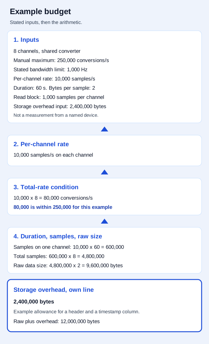
The worked example uses these inputs: 8 channels, a shared converter, a manual maximum of 250,000 conversions/s, a stated bandwidth limit of 1,000 Hz, a per-channel rate of 10,000 samples/s, a duration of 60 s, 2 bytes stored per sample, a read block of 1,000 samples per channel, and storage overhead of 2,400,000 bytes.
| Field | What you write | Example input |
|---|---|---|
| Channel count | Channels this task will store | 8 |
| Architecture | Shared converter, or one converter per channel | Shared converter |
| Manual maximum | Conversions/s if shared; samples/s on each converter if separate | 250,000 conversions/s |
| Stated bandwidth limit | Highest frequency you are treating as present, in Hz | 1,000 Hz |
| Per-channel rate | Samples/s on each channel | 10,000 samples/s |
| Duration | Seconds the file must cover | 60 s |
| Bytes stored per sample | Width of one stored sample in your file | 2 |
| Read block | Samples per read, and whether that count is per channel | 1,000 samples per channel |
| Storage overhead | Bytes for header, timestamps, or a second copy | 2,400,000 bytes |
What belongs on the sample and storage sheet?
Copy the architecture and the maximum from the manual for the module you will run. Write the bandwidth limit, the per-channel rate, the duration, the bytes per sample, the read block, and the overhead yourself. The result rows below are arithmetic from those cells. When the manual is silent, leave the matching cell blank.
The example column is filled so the arithmetic can be checked. It is not a reading from a named device, and it is not a limit you should copy onto a different module.
Takeaway: Copy the manual’s architecture and maximum, and leave a cell blank when that manual is silent.
What rate applies to each channel?
NI-DAQmx, in the Sampling Rate section updated 30 July 2026, defines the sampling rate as the speed at which a device acquires or generates a sample on each channel. Traditional NI-DAQ called that speed the scan rate. The number in the per-channel rate row is that kind of rate: one channel, not the sum of the task.
The same NI section illustrates point density with a generated 1 Hz signal: 1,000 points per cycle at 1,000 S/s, set beside 10 points per cycle at 10 S/s. Those two rates are NI’s picture of a generated cycle. They are not a maximum for your module. In the worked example, 10,000 samples/s across a stated 1,000 Hz limit is 10 samples in each cycle of that limit. Ten is the example’s choice of point density. Edit the rate cell and the later rows move with it.
DATAQ’s sample-rate tutorial says a sampling rule is usable only when the signal being digitized is bandwidth-limited, and that this limit has to be stated. The bandwidth row is that statement, in hertz. This page does not design the filter that would enforce the limit.
Hioki’s note updated 4 June 2025 says a higher sampling rate provides more detail and requires more storage and processing power, while a lower rate saves those resources and can leave out detail. Hold every example input still and change only the per-channel rate to 100,000 samples/s. The shared converter then sees 800,000 conversions/s, which is past the example manual maximum of 250,000, and the raw size becomes 96,000,000 bytes. Same sheet, one input edited.
Takeaway: Enter a per-channel rate, and pair it with a bandwidth limit you can write in hertz.
When does the total conversion rate fail?
The published rate is per channel. The total-rate test follows the architecture the manual names.
On a shared converter, the channels take turns through one converter. Total conversions per second equal the per-channel rate times the channel count. With the example inputs, 10,000 times 8 is 80,000 conversions/s. The example manual maximum is 250,000 conversions/s, and 80,000 is within 250,000, so this stated case passes. Swap only that maximum to 50,000 conversions/s and 80,000 is past it, so the condition fails. The next edit is a lower rate, fewer channels, or a different architecture from the manual.
On one converter per channel, each converter runs at the per-channel rate. The check is that rate against the maximum written for each converter. A separate example input, used only for this architecture, sets that maximum at 50,000 samples/s. Then 10,000 is within 50,000. Storage still multiplies by the channel count. Channel-count division is the shared-converter test. The per-channel card compares 10,000 with 50,000.
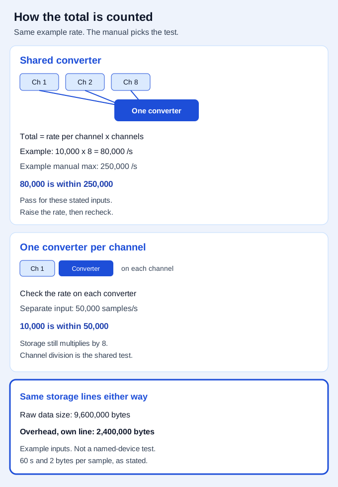
Takeaway: Multiply by the channel count for a shared converter. Compare the per-channel rate with each converter’s maximum when every channel has its own converter.
What does the read-block size change?
The read-block size is how many samples the program asks for on each read. Write whether that count is per channel or for the whole scan. In the example the block is 1,000 samples per channel, so the time between reads is 1,000 divided by 10,000 samples/s, which is 0.1 s. Each channel is read 600,000 divided by 1,000, which is 600 times, across the 60 s record.
If the software field counts every channel in the scan, divide the block by the total sample rate, per-channel rate times channel count. A block of 8,000 samples for all 8 channels at 10,000 samples/s per channel is the same 0.1 s. Match the divisor to the field you actually set.
The raw sample count stays 4,800,000 when every sample is returned once. A larger block means fewer reads. The duration row is still 60 s. The block row is 0.1 s of one channel in this example.
Common mistake: Treating the read-block size as the length of the recording. A block of 1,000 samples is one read. The file length is the duration row.
Takeaway: Use the block size to plan how often the program must read, and use the duration to plan the file.
How many samples and how many bytes?
Samples on one channel equal the per-channel rate times the duration. In the example, 10,000 times 60 s is 600,000. Total samples equal that count times the channels: 4,800,000. Raw data size equals total samples times the bytes stored per sample: 4,800,000 times 2 is 9,600,000 bytes.
Storage overhead stays on its own line at 2,400,000 bytes for this example. That figure is the example’s allowance for a file header and a separate timestamp column. Adding the raw line and the overhead line gives 12,000,000 bytes. Keep the overhead visible when you also write the sum.
| Result | How the example is computed | Example result |
|---|---|---|
| Samples in one cycle of the stated limit | 10,000 / 1,000 Hz | 10 |
| Total conversion rate | 10,000 × 8 | 80,000 conversions/s |
| Shared-converter condition | 80,000 against the 250,000 input | Within the example limit |
| Per-converter condition | 10,000 against a separate 50,000 samples/s input | Within that example limit |
| Time between reads | 1,000 / 10,000, block counted per channel | 0.1 s |
| Reads per channel | 600,000 / 1,000 | 600 |
| Samples per channel | 10,000 × 60 s | 600,000 |
| Total samples | 600,000 × 8 | 4,800,000 |
| Raw data size | 4,800,000 × 2 bytes | 9,600,000 bytes |
| Storage overhead | Stated on its own line | 2,400,000 bytes |
| Raw plus overhead | 9,600,000 + 2,400,000 | 12,000,000 bytes |
Hioki’s 4 June 2025 note also describes recorder behavior that samples quickly and stores less: an envelope mode that keeps minimum and maximum at a slower rate, and a dual-sampling mode on the MR6000 that keeps a fast stream and a slow stream. Those descriptions belong to that vendor’s recorders. If your manual splits the acquisition rate from the rate written to disk, the sample-count rows use the stored rate, and the acquisition rate keeps its own cell.
Takeaway: Raw bytes are total samples times bytes per sample. Overhead is the next line.
Where does this budget stop?
The sheet covers the actual sample rate, the read-block size, the channel architecture, the duration, and the data budget. Range, shunt, and isolation are earlier checks, on the DAQ versus oscilloscope page. A trace that repeats another channel is a separate hardware-artifact diagnosis. Matching clocks across two devices is a separate synchronization job. The bandwidth cell records the limit you are using. Filter design sits outside this page.
Other instrument notes are on the blog. Sensor and DAQ pieces are under sensors and DAQ.
Takeaway: Stop when each result row is filled from the inputs, or still blank because the manual has not answered it.
Method and sources
Compiled on 12 October 2026 from the public pages listed at the end of this article. The NI-DAQmx Sampling Rate page shows an update date of 30 July 2026 and is used for the per-channel definition and for NI’s 1 Hz point-density illustration. DATAQ’s tutorial is used for the requirement that a bandwidth limit be stated. The archived DATAQ text does not show a publication date. Hioki’s note shows an update date of 4 June 2025 and is used for the storage tradeoff and for that vendor’s envelope and dual-sampling descriptions. Example numbers are stated inputs for the worksheet. This site did not measure a device. The bench picture is an illustration. National Instruments product names appear only where those public pages name them. Nothing here is an NI or Emerson document, and nothing here is investment advice.