Strain-Gauge mV/V Output Converted to Load

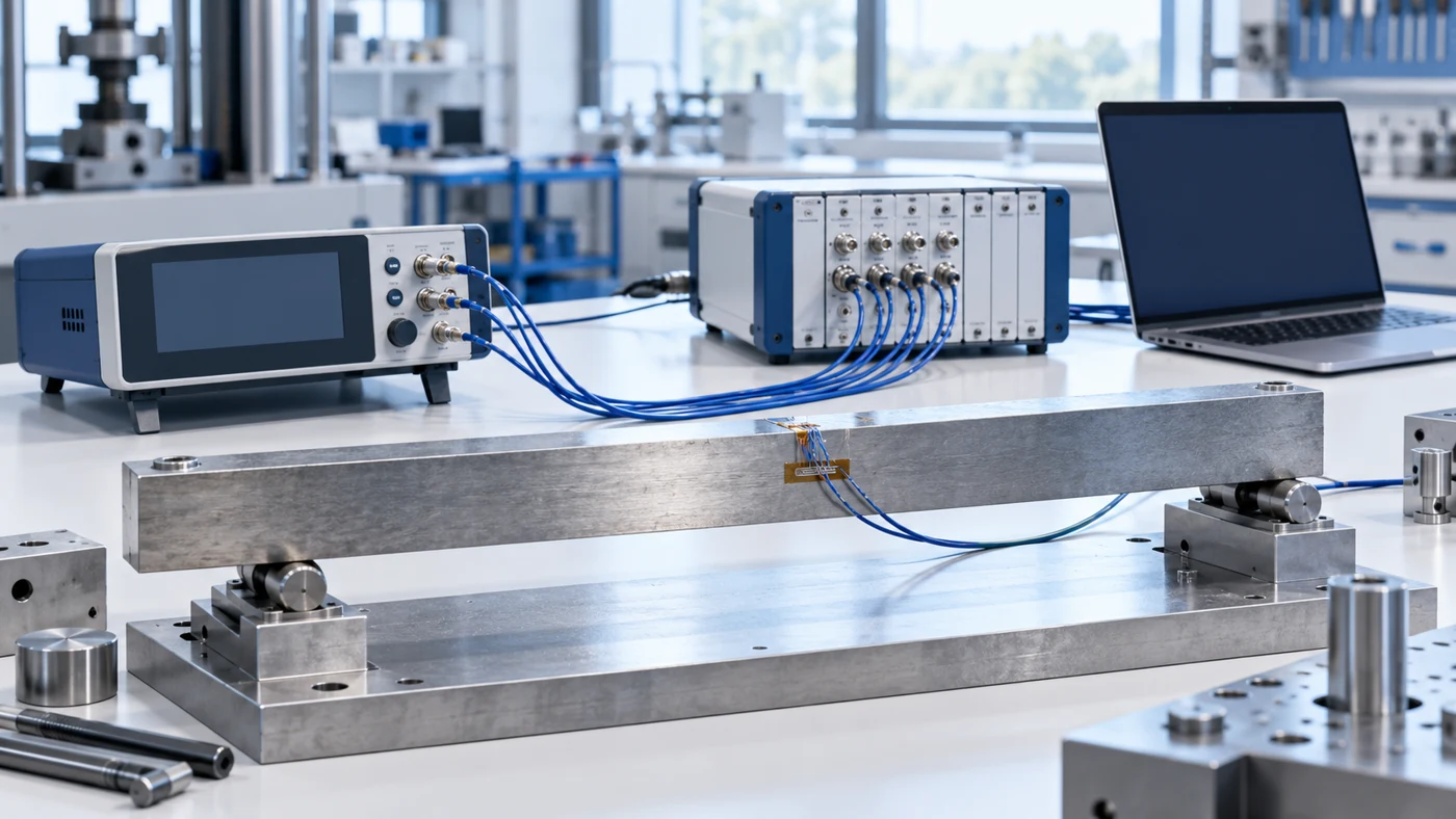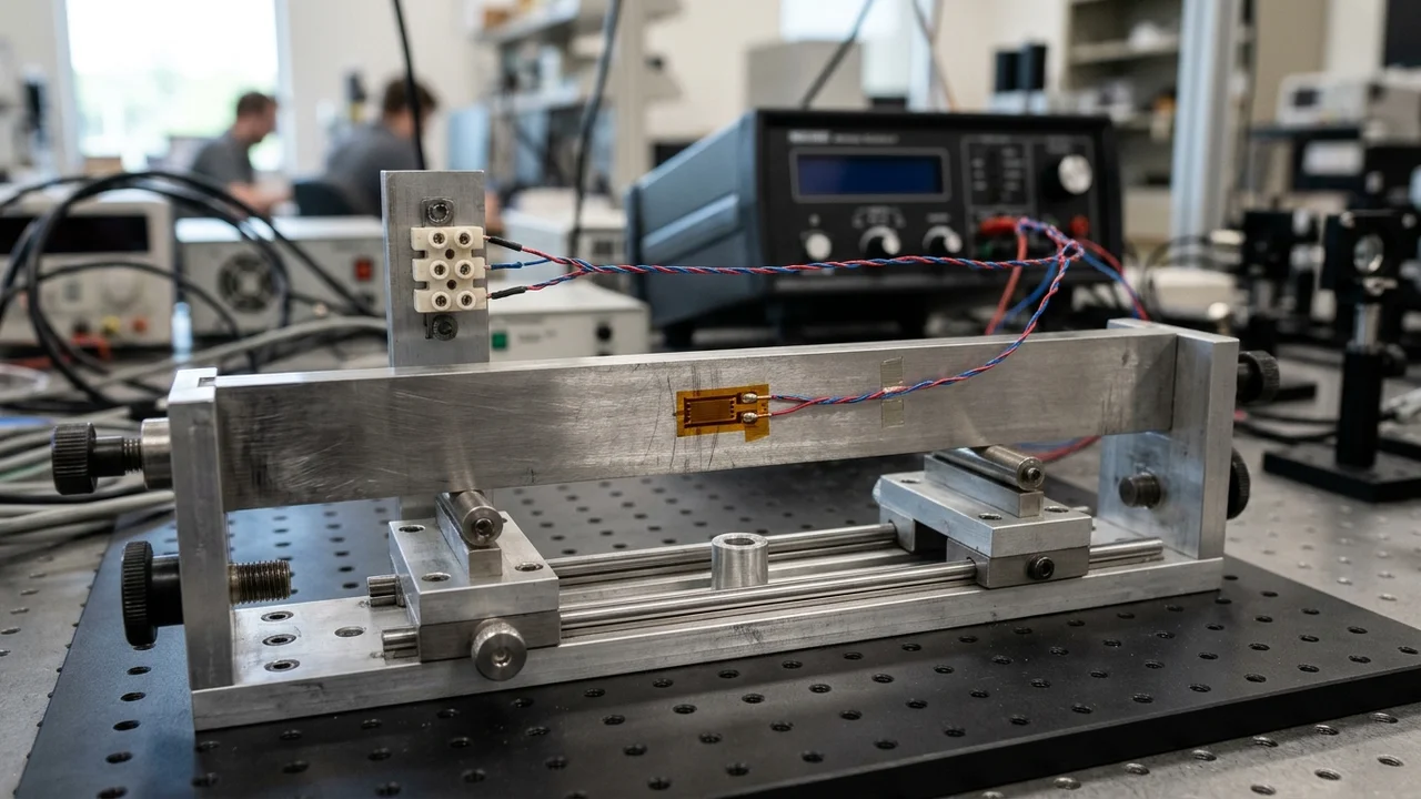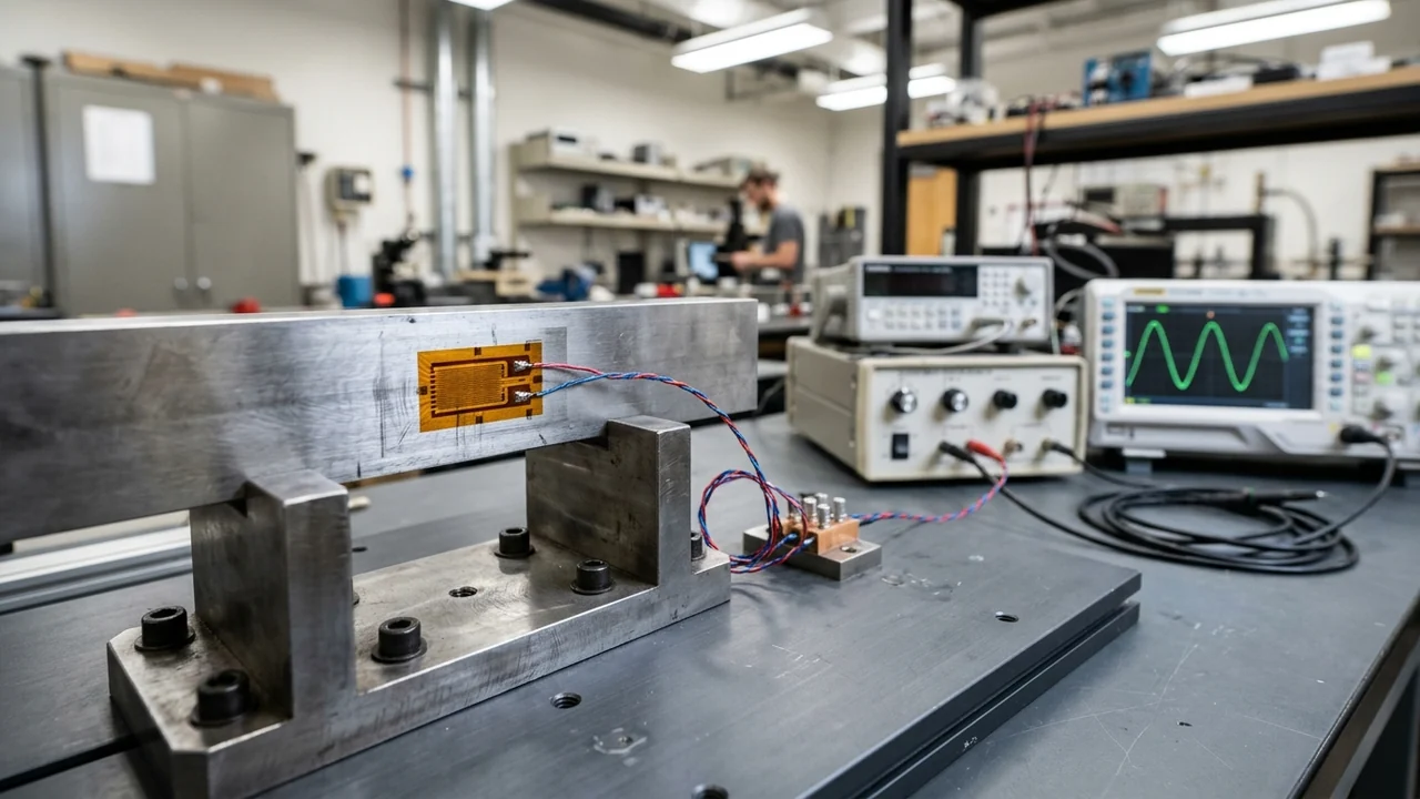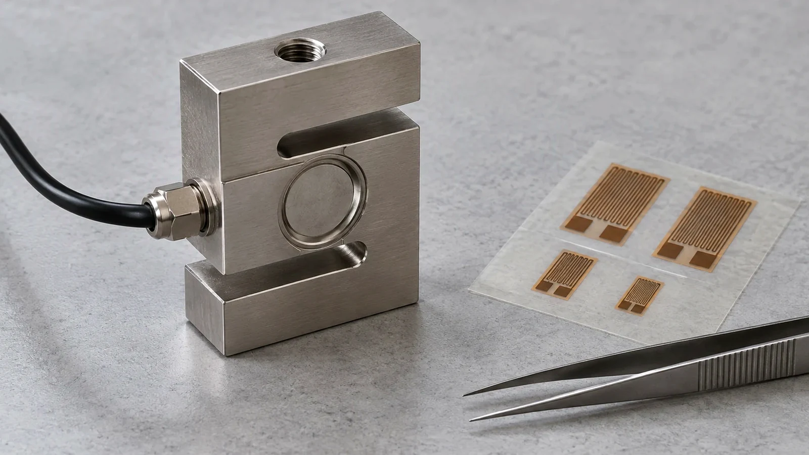
Converting a millivolt bridge signal into engineering force or mass is a core scaling task across sensors and data acquisition systems. Load cells are much simpler than strain gauge bridges because their relationship to load does not require additional detail of how its internal bridge elements are arranged, its Gauge Factor, or the Poisson’s ratio of the material it is applied to; the only important considerations for resolving the load cell are its rated output (mV/V), excitation voltage, and rated capacity.

Maximizing Value at NI is an independent engineering publication and is not affiliated with or endorsed by National Instruments or Emerson; learn more about this publication.

The Core mV/V-to-Load Conversion Equation

When scaling a strain gauge load cell sensor for strain gauge weight measurement, the sensitivity of a bridge network or load cell is how much the bridge output voltage changes relative to 1V of bridge excitation and expressed in millivolts of Vo per volt of excitation Vex (mV/V), usually referred to as the gauge or cell Rated Output and denoted by Vr = Vo / Vex. The full-scale output of a strain gauge bridge or load cell sensor at its full rated load (100%) is the product of the gauge Rated Output (mV/V) and applied excitation voltage Vex.

There are normally two sensor measurements used to resolve strain or load: the sensor bridge output signal Vo and the sensor bridge excitation Vex, and using sensor specifications and these two measurements, the applied strain or load can be resolved from the bridge output signal. In the SCXI-1520 User Manual, VCH is the measured voltage of the signal, VEX is the excitation voltage, and Vr is the voltage ratio used in the voltage to strain conversion equations and defined as Vr = (VCH(strained) – VCH(unstrained)) / VEX.

In OIML R 60-1:2021 (E) Section 1 Introduction, load cells comprise a distinct element or module within other complex instruments and do not produce distinct quantitative values that are inherently identified or associated with denominations or units; the data that can be extracted from a load cell is simply a measurement of change in the output of the load cell in relation to the input. Under section 3.1.3.1, a load cell is a measuring transducer that will produce an output in response to an applied load which may be converted by another device into measurement units such as mass, and an analogue-passive load cell may utilise passive electronics (e.g. strain gauges) and passive temperature compensation elements.

Within load cell metrology, load cell output is the measurable quantity into which a load cell converts the measured input quantity, maximum capacity (Emax) is the largest value of a quantity expressed in units of mass which may be applied to a load cell, minimum dead load (Emin) is the smallest value of a quantity (expressed in mass units) that may be applied to a load cell, and maximum measuring range = (Emax – Emin). The weight indicators and weight transmitters usually have a standard power supply value of 5VDC or 10VDC, while load cell input and output resistance is typically between 350 and 400 Ohm or between 700 and 800 Ohm, maximum static load is normally between 120% and 150% of the full scale, and breaking load is usually between 250% and 300% of the full scale.

Step-by-Step Worked Conversion Examples

In a worked example for a compression load cell with six connection wires (sense ±, excitation ±, and signal ±), the transducer is specified by its manufacturer with Rated Output: 2.0mV/V, Rated Excitation: 10V DC (15V Maximum), Rated Capacity: 50,000 lbs/square-inch, Safe Overload Level: 150% of Full-Scale, and Operating Temperature Range: -65°F to 200°F.

When the cell output is Vo = 0.0035V (3.5mV) on a load cell whose rated output is 2mV/V and excitation is 10V, 100% of load corresponds to 10V * 2mV/V = 20mV (50000lbs/in2 or 50000psi), and the load at Vo = 3.5mV is simply 3.5 / 20 * 50000psi = 8750lbs/square-inch, or 17.50%.

Additionally, this load cell may be over-loaded up to 75000psi (150% of full-scale) and Vo = 30mV for a load of 75000psi with 10V of excitation because its safe overload limit extends to 150%.

How Gauge Factor and Bridge Physics Produce mV/V

Engineers asking what is the gauge factor of a load cell should examine how individual strain gauge factor and transverse sensitivity relate to the complete bridge transducer. Under ASTM E0251-20A, gage factor is the transfer function of a strain gage that relates resistance change in the strain gage and strain to which it is subjected, and accuracy of strain gage data can be no better than the accuracy of the gage factor; under Clause 1.5, these test methods do not apply to transducers, such as load cells and extensometers, that use bonded resistance strain gages as sensing elements.

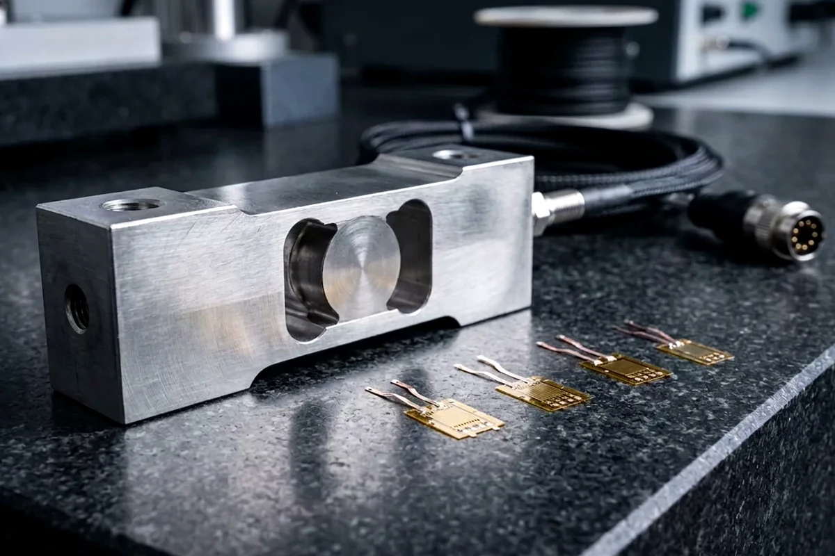
In the construction of load cells (see sections 1 and 2.1), a strain gauge is an analogue resistive element that is attached to a load cell structure and that changes resistance depending on the deformation of the load cell structure when compression or tension forces are applied to the load cell. Most load cells will have 4 or 6 leads and already have bridge completion and temperature compensation built-in; internally, a load cell will contain some permutation of quarter, half, or full-bridge circuitry, but this detail is irrelevant to the load computation and is not usually provided by the load cell manufacturer.

Assuming the strain gage has a gage factor of 2.0, the output of a strain gage bridge circuit is (0.5 µV / V / µɛ) X N, where N is the number of active arms; for a quarter-bridge (N = 1), the output of the circuit is (0.5 µV / V / µɛ) X 1, and if the supplied excitation voltage is 10 VDC, then the output will be 5 µV per µɛ. In load cells and other transducer applications, the OEM manufacturer typically chooses to use a full-bridge configuration, and in the case of a full-bending bridge, the output of the bridge circuit will be determined by (0.5 µV / V / µɛ) X 4, so if the excitation voltage is 10 VDC, then the output will be 20 µV per µɛ.

Bridge Circuit Type	Active Bridge Factor	Output Sensitivity Formula	Example Bridge Output
Quarter-Bridge Circuit	N = 1 active arm at gage factor 2.0	(0.5 µV / V / µɛ) X 1	5 µV per µɛ at 10 VDC excitation voltage
Full-Bending Bridge	N = 4 active arms in full-bridge configuration	(0.5 µV / V / µɛ) X 4	20 µV per µɛ at 10 VDC excitation voltage
Full Poisson Axial Bridge	N = 2 + (2 X ν) where ν is Poisson’s ratio	N = 2 + (2 X ν) active arms	N = 2 + (2 X ν) where ν is Poisson’s ratio of the material

Most load cells and transducers are manufactured so the full-scale rated mechanical load will produce 1000 µɛ at the gage locations, where the full-scale output is calculated as 0.5 X 10 X 1000 X 4 = 20,000 µV or 20 mV, which is where the common expression of 2 mV/V for 1000 µε for this device originates. Not all full bridges are N = 4, however: for a full Poisson (axial) bridge, N = 2 + (2 X ν) where ν is Poisson’s ratio of the material, and in circumstances where instrumentation does not provide bridge completion and expects to receive only a full bridge, a single strain gage may be configured with a bridge completion module to create a full bridge where N = 1.

Error Sources: Cable Voltage Drop, Zero Offset, and Metrological Limits

In the case of a full-bridge circuit, the leadwire resistance is in the bridge power and output leads rather than in the bridge arms, and the resistance in the power leads reduces the voltage applied to the bridge proper and attenuates the output signal accordingly. In ratiometric measurements, the excitation voltage is continuously sensed by precision circuitry on the modules and used to drive the reference input of the ADC so the modules return data as a ratio of the bridge output voltage and the excitation voltage, and with feedback remote sensing, you connect extra sense wires to the point where the excitation voltage wires connect to the bridge circuit.

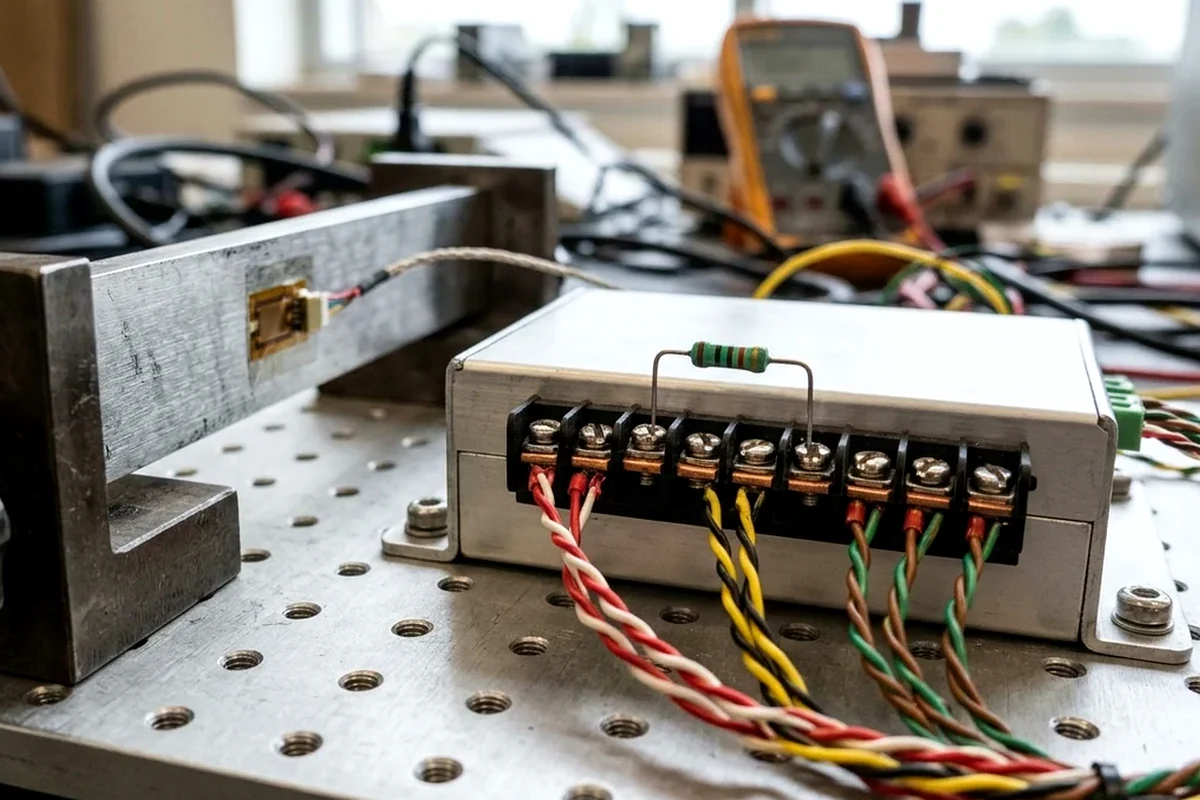
If you connect the remote sense signals directly to the bridge resistors, the NI 9237 senses the actual bridge voltage and eliminates the gain errors caused by the resistance of the EX+ and EX- leads, while its 150 mW limit allows you to power four 350 Ω half bridges at 5.0 V, four 350 Ω full bridges at 3.3 V, or four 120 Ω half bridges at 2.5 V excitation. Deflection at nominal load comes within a range between 0,2 mm and 1 mm (for example, 0,5 mm in an AZL load cell), and load cells typically have 4 or 6 wires: 6-core cables include 2 wires called reference wires (Sense + and Sense-) to compensate for voltage drops, whereas 4-wire load cells are calibrated and thermally compensated and require a shielded cable with a significant cross-section (at least 1 mm2).

Parameter Category	Physical Mechanism or Definition	Quantitative Value or Example	Metrological or Wiring Rule
Deflection and Wiring	Deflection at nominal load and lead wire configuration	0,2 mm to 1 mm deflection (0,5 mm in AZL); 4 or 6 wires	Use 2 reference wires (Sense + and Sense-) or shielded cable of at least 1 mm2
Unloaded Offset vs Tare	Non-zero unloaded output versus constant container tare weight	Fails to indicate 0% load with no load applied	Null unloaded offset before measurements and do not combine Tare with Offset
Combined Error Envelope	Sum of 3 errors: linearity, hysteresis, and temperature effects	10000 kg full scale with 0,05% combined error gives 5 kg error	Rated output in mV/V is output in mV at maximum load divided by supply in V
Type Evaluation MPE	Apportioning factor pLC chosen and declared by manufacturer	0.3 to 0.8 (0.3 ≤ pLC ≤ 0.8), or 0.7 assumed if not specified	Maximum Permissible Errors are pLC × 0.5 v, pLC × 1.0 v, and pLC × 1.5 v

Load cells commonly fail to indicate exactly 0% load with no load applied, so you should Null the unloaded offset using module controls to remove it prior to taking measurements and prior to Load Calibration, and do not combine Tare with Offset because if you erroneously use Null Offset to remove Tare weight, your subsequent load cell measurements will be in error. Modern instruments usually include a Tare control to automatically remove tare weight (a constant load of common/nonvariable elements between loads, like the weight of its container or its shipping materials) from the load cell measurement so that the sensor Vo will be automatically corrected for both non-zero offset and/or tare such that Vo = Vo(loaded) - Vo(ioffset) - Vo(tare).

Load Calibration does not calibrate the instrument itself, but the load cell it connects to, by rescaling the indicated load using only Software Gain (load cells do not usually disclose their internal Gauge Factor); null any unloaded load cell offset to zero and allow the instrument module to warm-up several minutes prior to attempting Load Calibration, which should not include any defined tare.

Combined error is the sum of the 3 errors (linearity, hysteresis and effects of temperature); for a load cell with a 10000 kg full scale and a combined error equal to 0,05%, one would expect a maximum error of 5 kg, while the rated output, expressed in mV/V, is the output value in mV that the load cell returns when the maximum load is applied, divided by the power supply voltage in V units. In OIML classification, the maximum number of load cell intervals is stated in units of 1 000, where 3 represents 3 000 and 1.5 represents 1 500, for example C3.

On type evaluation (Table 4), the apportioning factor pLC shall be chosen and declared (if other than 0.7) by the manufacturer and shall be in the range of 0.3 to 0.8 (0.3 ≤ pLC ≤ 0.8), with Maximum Permissible Errors (MPE) of pLC × 0.5 v, pLC × 1.0 v, and pLC × 1.5 v, and if the apportioning factor pLC is not specified on the certificate then the value 0.7 shall be assumed. Mandatory markings and documentation include Maximum capacity as Emax = (in units g, kg, t), Minimum dead load as Emin =, Safe load limit as Elim =, Minimum load cell verification interval as vmin, pLC if not equal to 0.7, and output rating, input impedance, supply voltage, cable details, and mounting torque.

Configuring Load Cell Readouts and DAQ Channels

Selecting and scaling load cell readouts depends on how the ADC architecture resolves the ratiometric bridge signal. A modern instrument takes Vo and Vex voltage measurements to determine the load using its 16-bit or higher bipolar ADC to determine a count = Vin * Gain * 32768 / Reference + 32767; for example, the Acromag TT351-0700 first measures Vex relative to a fixed reference Vref2 and gain of 1 to solve for the excitation voltage Vex = (count - 32767) * Vref2 / 32768. The Acromag TT351-0700 also measures the cell Vo relative to a variable ratiometric reference Vref1 derived from Vex; with a rated output 2mV/V and overrange up to 150%, Vo(max) = 1.5 * 2mV/V * Vex, and it sets Gain to the largest of 1, 2, 4, 8, 16, 32, 64, or 128 < Vref1 / Vo(max) and solves for Vo = (Vo(count) – 32767) * Vref1 / (Gain * 32768).

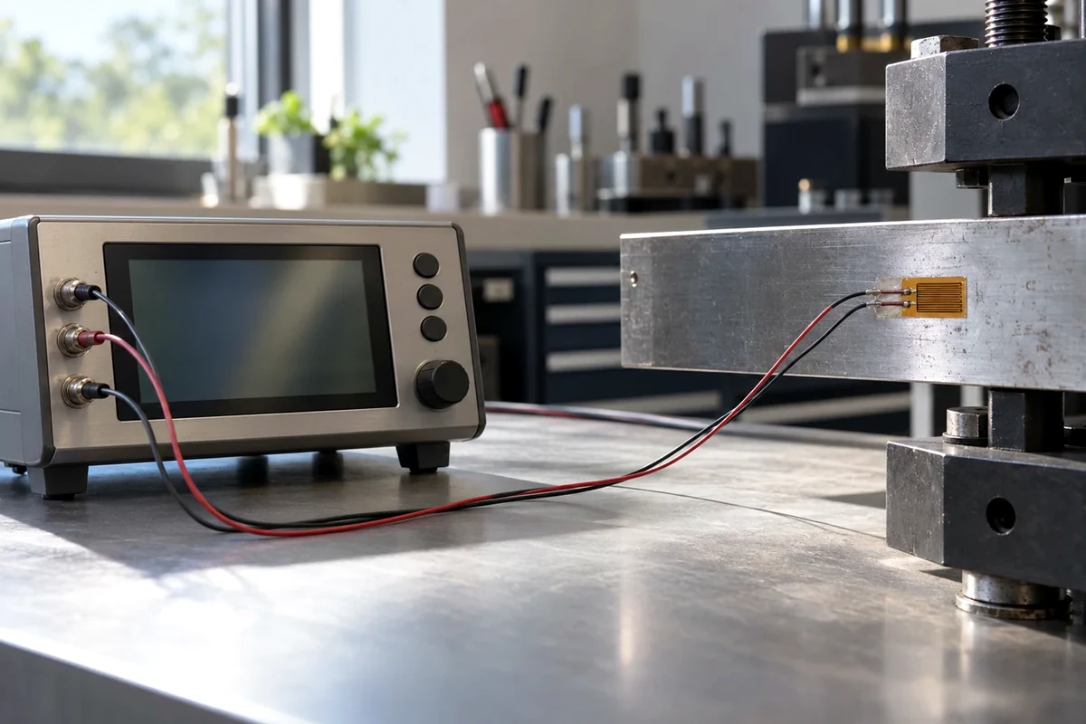
For high-speed bridge data acquisition, the NI 9237 has 4 analog input channels, internal half and full bridge completion (external quarter bridge), 24 bits Delta-Sigma ADC resolution, 50 kS/s maximum sampling rate, a typical input range of ±25 mV/V, a scaling coefficient of 2.9802 nV/V per LSB, internal voltage of 2.5 V, 3.3 V, 5.0 V, and 10.0 V with 150 mW maximum internal power, and external voltage of 2 V to 10 V supplies. In the NI 9237 Table 1 Accuracy (where Range equals 25 mV/V), calibrated typical accuracy at 25 °C (±5 °C) is 0.05% and 0.05%, maximum accuracy from –40 to 70 °C is 0.20% and 0.25%, gain drift is 10 ppm/°C maximum, and offset drift is 0.6 µV/V per °C at 2.5 V excitation, 0.5 µV/V per °C at 3.3 V excitation, 0.3 µV/V per °C at 5 V excitation, and 0.2 µV/V per °C at 10 V excitation.

The IEEE 1451.4 standard defines the method for encoding TEDS information, and Table 4 shows an example of a TEDS for a load cell with Measurement Range ±100 lb, Electrical Output ±3 mV/V, Bridge Impedance 350 Ω, Excitation Nominal 10 VDC, Excitation Minimum 7 VDC, Excitation Maximum 18 VDC, and Response Time 333.33 μs. You can use the SCXI-1314T terminal block to read TEDS load cells with the SCXI-1520.

Benchtop Indicator and Transmitter Scaling Methods

• Under Method I (Scaling Without Simulating a Known Load), the 3 parameters are RDG SC (Reading Scale), RDG OF (Reading Offset), and DEC PT (Decimal Point), where RDG SC = display span / ((sensor's mV/Voutput) (natural gain)); for display span = 200 – 0 = 200, sensor’s output = 100 mV / 10V EXC = 10 mV/V, and meter’s natural gain = 10000 (obtained from Table 8-1), RDG SC = 200 / (10 x 10000) = 0.002.
• When you simulate two loads on the transducer and record the meter display as INPUT1 and INPUT2, normally the two points that are calibrated are the no load condition and 3/4 full scale; if you simulate no load and the display indicates 13, and when you simulate 160 PSI the display indicates 80567, you enter INPUT1: 13, READ 1: 000000, INPUT2: 80567, and READ 2: 000160.
• Similarly, if you simulate no load and the display indicates –55.6, and when you simulate 4.0000 pounds the display indicates 16136.6, the data entered into the 2-point scaling IN.SC.OF method is INPUT1: –55.6, READ 1: 00000.0, INPUT2: 16136.6, and READ 2: 04000.0.
• The P3 Strain Indicator and Recorder features a 24-bit sigma-delta converter, dynamic range of ±31,000 µƐ (±1 µƐ resolution) at Gage Factor = 2.000, gage factor range 0.500 to 9.900, automatic calculation of mV/V, and linear scaling for engineering units including µƐ, g, rpm, hp, mV/V, lbf, m, deg, psi, lb, s, rad, ksi, kg, A, oz, GPa, in, N, mV, MPa, mm, V, m/s2, Pa, mil, Ω, and ton.
• The Model D4 Data Acquisition Conditioner provides a strain range of ±31,000 µƐ at GF = 2.000 (±15.5 mV/V), resolution of ±1 µƐ at GF = 2.000 (±0.0005 mV/V), measurement accuracy of ±0.1% of reading ±3 counts (Instrument Gage Factor = 2.000), gage factor control range 0.500 to 9.900, and 1.5 VDC nominal bridge excitation.
• For industrial fieldbus and analog integration, the TLB4 PROFINET IO digital weight transmitter features a 6 digit red LED display (8 mm height), 4 independent reading channels for load cells, OIML R 76:2006 approved class III for 10,000 divis. at 0.2μV/VSI, a 4 channels 24bit (16000000 points) 4.8 kHz A/D converter, and MODBUS-RTU registers with the mV/V value of the analog input channels.
• The TLC analog weight transmitter, with dimensions of 45 x 26 x 11 mm in the board-only version, IP67 ABS enclosure version, or diameter of only 20mm, provides analog output in current (4-20 mA) or voltage (0-10 VDC), connection of up to 4 load cells in parallel, rated output selection with mini switches in a range between 1 mV/V and 3 mV/V, and a 12-turn potentiometer for zero and full-scale adjustment.

Sources

• Acromag — Introduction to Strain and Strain Measurement Technical Whitepaper
• Vishay Micro-Measurements — Use of the Full Wheatstone Bridge in Experimental Stress Analysis
• Vishay Micro-Measurements — Shunt Calibration of Strain Gage Instrumentation Technical Note
• Vishay Micro-Measurements — Strain Indicator, Recorder, and Data Acquisition Conditioner Specifications
• International Organization of Legal Metrology — Metrological Regulation for Load Cells
• National Instruments — Engineer Guide to Accurate Sensor Measurements and Bridge Module Manuals
• Omega Engineering — High Performance Strain Gage Indicator User Guide
• LAUMAS — Load Cell Technical Features Guide and Weight Transmitter Datasheets