Dynamic Versus Static Strain Gauge Measurement: Range, Fatigue, and Zero Drift

Treating a strain gauge’s catalog maximum elongation rating as its usable cyclic operating span causes premature fatigue damage, unstrained zero-shift, tensile waveform distortion, and open-circuit tab failure well below the static strain limit. Conversely, applying a high-output dynamic gauge alloy or dynamic bridge excitation power density to a long-term static test introduces severe thermal apparent-strain drift and adhesive creep that mask real structural deformation.

Separate static from dynamic strain gauge specifications across four physical boundaries: bound alternating cyclic strain using Vishay Micro-Measurements Tech Note TN-508-1 fatigue curves (±1,200 to ±2,500 με for 10^6–10^8 cycles at a 100 με zero-shift criterion) rather than monotonic elongation limits (±15,000 to ±200,000 με); select Self-Temperature-Compensated (S-T-C) Constantan (A-alloy, < +65°C) or Modified Karma (K-alloy, up to +260°C) with DC or carrier coupling for static zero stability versus Isoelastic (D-alloy, GF ≈ 3.2) or Karma with AC coupling for dynamic endurance; restrict solder to the lower third of copper tabs with intermediate terminal strips; and scale bridge excitation power density P'_G = E_B^2 / (4 × R_G × A_G) from 1–2 W/in² (1.6–3.1 kW/m²) for high-accuracy static steel tests up to 5–10 W/in² (7.8–16 kW/m²) for dynamic tests per Tech Note TN-502.

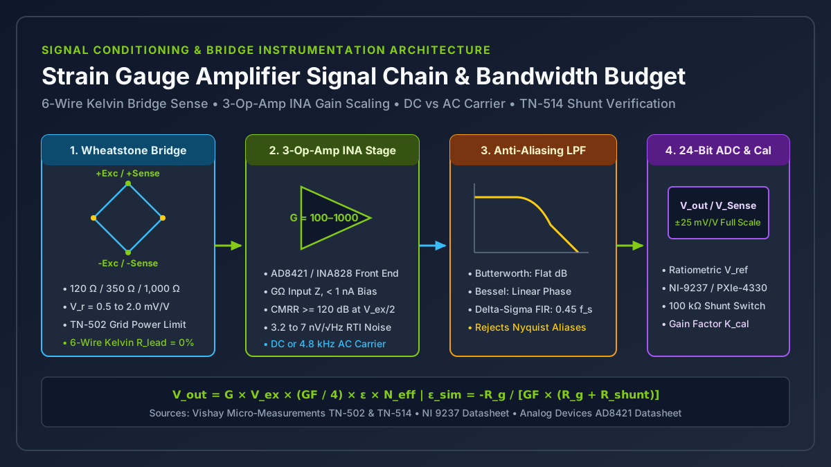
This engineering comparison belongs to the Sensors and DAQ documentation hub. It builds on the fundamental resistance-to-strain transfer function (ΔR/R = GF × ε) covered in our strain gauge basics guide and pairs with our strain gauge amplifier and signal conditioning bandwidth guide, which derives instrumentation amplifier gain, 6-wire Kelvin remote sense, and anti-aliasing filter responses. Maximizing Value at NI is an independent technical publication (about this site) not affiliated with National Instruments (NI) or Emerson.

Specification Dimension	Static Sustained Load / Long-Term Hold	Combined Static-Dynamic Measurement	Purely Dynamic Cyclic / Transient Impact
Measurand & Baseline Requirement	Constant or stepwise deformation (0 Hz DC); absolute zero reference must hold over hours, months, or years (TN-505-4)	Mean static load offset (ε_mean) plus alternating cyclic strain (±ε_alt) measured simultaneously (TN-508-1)	Alternating peak-to-peak amplitude (Δε_p-p), frequency spectrum, or transient pulse; slow baseline drift rejected
Governing Strain Range Limit	Monotonic static elongation limit: ±1.5% (±15,000 με) on W-backing, ±3–5% (±30,000–50,000 με) on EA/CEA/SGD, ±20% (±200,000 με) on EP	100 με fatigue zero-shift curve (±1,300 με at 10^6 cycles on CEA; ±2,000–2,200 με at 10^7 cycles on SK/WK)	100 με zero-shift (WK/EA) or 300 με zero-shift / onset of tensile super-sensitivity (±2,500 με at 10^7 cycles on WD)
Preferred Foil Alloy & Carrier Series	CEA / EA / Omega SGD (A-alloy < +65°C); WK / SK / EK (K-alloy for multi-month stability or up to +260°C); EP (P-alloy post-yield)	WK / SK / EK (K-alloy matched S-T-C for low zero drift + high fatigue life); EA / WA / SA for moderate cycles (< 10^6)	WD / SD / ED (Isoelastic D-alloy, GF ≈ 3.2, no S-T-C) or WK / TK with pre-attached beryllium-copper leads
Dominant Error & Failure Mechanism	Thermal output ε_T/O (TN-504-1 Eq. 1), Constantan drift > +65°C, glueline creep, and moisture shunting (< 500 MΩ)	Cold-work unstrained resistance shift (> 100 με zero-shift) corrupting the static mean load baseline (TN-508-1)	Foil micro-crack tension peak distortion (“super-sensitivity”) and copper-tab / solder-fillet notch fatigue fracture (TN-508-1)
Excitation Power Density (TN-502, Thick Steel)	1–2 W/in² (1.6–3.1 kW/m²) for high static accuracy; 2–5 W/in² (3.1–7.8 kW/m²) for moderate accuracy	Bounded by the static baseline stability limit: 1–2 W/in² (high accuracy) to 2–5 W/in² (moderate accuracy)	5–10 W/in² (7.8–16 kW/m²) for high dynamic accuracy; 10–20 W/in² (16–31 kW/m²) for moderate accuracy
Signal Conditioning & Sampling Rate	DC-coupled bridge or 1.2–4.8 kHz AC carrier demodulator down to 0 Hz; low sample rate (0.1 Hz to 100 S/s)	Wideband DC-coupled bridge amplifier or high-speed carrier; 1 kS/s to 100 kS/s (StrainBlog, 11 Oct 2023)	AC-coupled (high-pass filtered) or pre-burst AutoZero wideband DC amplifier; 1 kS/s (cyclic) to 10 MS/s (ballistics/impact)

Takeaway: Never size a cyclic fatigue test from a datasheet’s “Maximum Strain” percentage; determine first whether your channel must preserve a DC zero reference over time (static or combined static-dynamic) or capture only alternating waveforms (purely dynamic).

Why Does Static Strain Gauge Range Differ from Dynamic Cyclic Fatigue Life?

Mechanical strain $\varepsilon = \Delta L / L$ is dimensionless and expressed in microstrain ($\mu\varepsilon$), where $1,\mu\varepsilon = 10^{-6},\text{m/m} = 0.0001%$ length change, $1,000,\mu\varepsilon = 0.1%$, and $10,000,\mu\varepsilon = 1.0%$. On a manufacturer specification sheet—such as DwyerOmega’s Strain Gage Technical Data (page E-7 for the SGD Series) or Vishay Micro-Measurements Tech Note TN-505-4 (Strain Gage Selection: Criteria, Procedures, Recommendations)—two completely different microstrain ratings appear side by side:

1. Maximum Strain (Static Elongation Range): The largest single monotonic tension or compression excursion the foil grid and backing carrier can undergo before physical necking, grid cracking, or bond shear failure. For general-purpose Constantan foil on a polyimide carrier (EA and CEA series with gauge length $\ge 0.125,\text{in}$ [$3.2,\text{mm}$]), the static elongation limit is $\pm 5%$ ($\pm 50,000,\mu\varepsilon$), or $\pm 3%$ ($\pm 30,000,\mu\varepsilon$) for shorter gauges and for the DwyerOmega SGD series ($5,\mu\text{m}$ Constantan foil on a $20,\mu\text{m}$ polyimide substrate with a $25,\mu\text{m}$ cover). For specially annealed Constantan (EP series, P-alloy), static post-yield elongation reaches $\pm 20%$ ($\pm 200,000,\mu\varepsilon$) on gauges $\ge 0.125,\text{in}$ ($\pm 10%$ under $0.125,\text{in}$).
2. Dynamic Fatigue Life (Cyclic Strain Range): The alternating strain amplitude $\pm\varepsilon$ at which a metallic foil grid survives a target number of load reversals ($N = 10^5, 10^6, 10^7,$ or $10^8$ cycles) before accumulating a permanent unstrained resistance shift (zero-shift) of $100,\mu\varepsilon$ ($300,\mu\varepsilon$ for dynamic-only WD gauges). Per Vishay Micro-Measurements Tech Note TN-508-1 (Fatigue Characteristics of Micro-Measurements Strain Gages), all metallic foils undergo cyclic strain hardening and slip-band micro-cracking at strain amplitudes between $\pm 1,000,\mu\varepsilon$ and $\pm 3,000,\mu\varepsilon$—just $0.5%$ to $10%$ of their monotonic elongation limit.

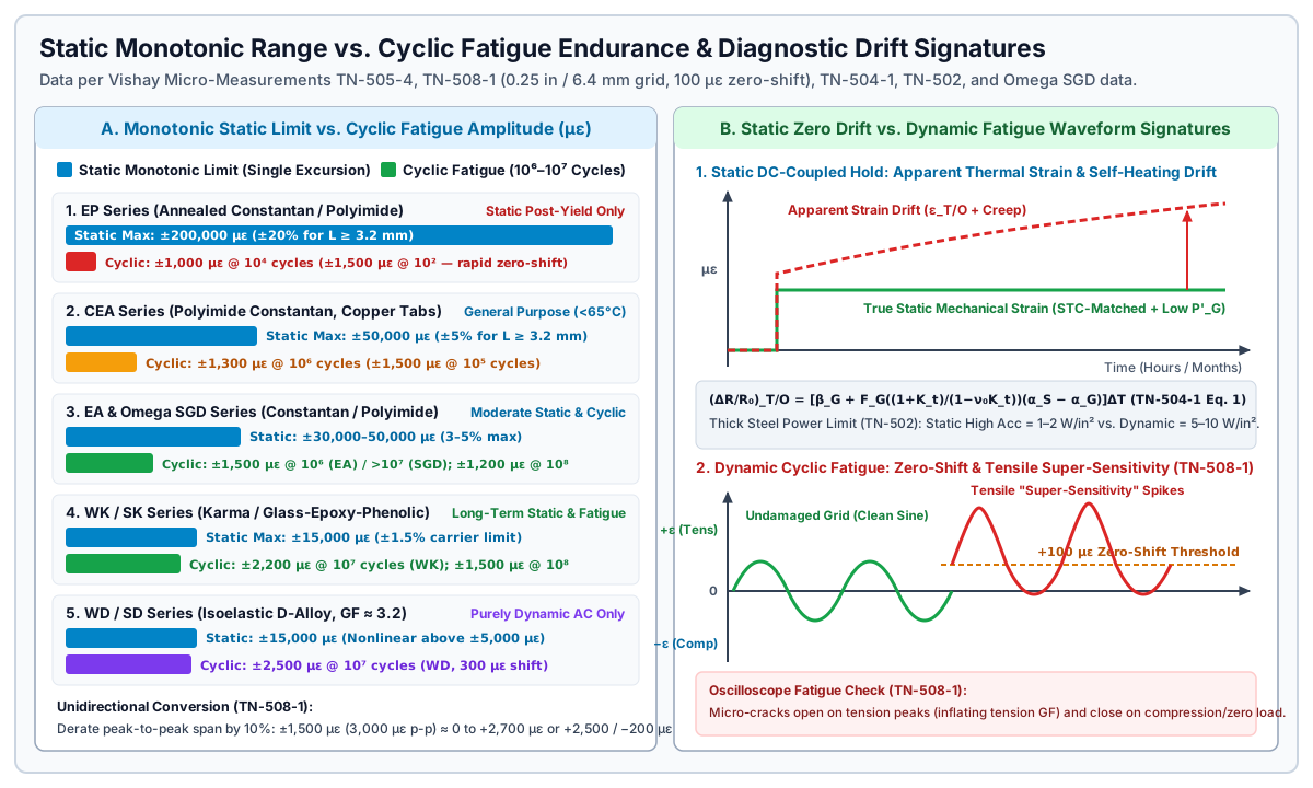
The table below compiles the side-by-side monotonic static limits and nominal fully reversed cyclic fatigue endurance values from Vishay TN-508-1 (Table 1, measured on $0.25,\text{in}$ [$6.4,\text{mm}$] gauges bonded to NAS-942 constant-stress beams), TN-505-4 (Section 2.3 selection chart, nominal for gauge lengths $\ge 0.125,\text{in}$ [$3,\text{mm}$]), and DwyerOmega Strain Gage Technical Data (page E-7):

Gauge Series	Foil Alloy & Nominal GF	Carrier Backing & Leads/Tabs	Service Temp Range (TN-505-4 / A05)	Static Max Strain (Monotonic)	Cyclic Strain @ 10^5 Cycles	Cyclic Strain @ 10^6 Cycles	Cyclic Strain @ 10^7 Cycles	Cyclic Strain @ 10^8 Cycles
EP (Vishay)	Annealed Constantan (P), GF ≈ 2.0	Flexible Polyimide (E), open-face	-75°C to +205°C (-100°F to +400°F)	±20% (±200,000 με, L ≥ 3.2 mm); ±10% (L < 3.2 mm)	Fails (±1,500 με @ 10^2; ±1,000 με @ 10^4)	Not rated (severe cyclic zero-shift)	Not rated	Not rated
CEA (Vishay)	S-T-C Constantan (A), GF ≈ 2.05	Encapsulated Polyimide, large copper-coated tabs	-75°C to +175°C (+65°C max on stacked rosettes)	±5% (±50,000 με, L ≥ 3.2 mm); ±3% (L < 3.2 mm)	±1,500 με	±1,300 με (±1,500 με w/ low-modulus solder)	Not rated for ≥ ±1,300 με	Not rated
EA (Vishay)	S-T-C Constantan (A), GF ≈ 2.05	Flexible Polyimide (E), open-face (or Option E/SE)	-75°C to +175°C normal (-195°C to +205°C short-term)	±5% (±50,000 με, L ≥ 3.2 mm); ±3% (L < 3.2 mm)	±1,800 με (TN-505-4)	±1,500 με	~±1,350 με (interpolated curve)	±1,200 με
SGD (DwyerOmega)	S-T-C Constantan (5 μm), GF = 2.0 ± 5%	Polyimide (20 μm base, 25 μm cover), tinned Cu ribbons/pads	-75°C to +200°C (-5°C to +120°C temp-compensated)	±3% (±30,000 με)	> ±1,500 με	> ±1,500 με	±1,500 με (> 10^7 cycles)	Not specified
WA / SA (Vishay)	S-T-C Constantan (A), GF ≈ 2.05	Glass-fiber epoxy-phenolic (W leads / S solder dots)	-75°C to +205°C normal (-195°C to +260°C on WA)	±2% (±20,000 με)	±2,000 με (WA in TN-505-4)	±1,800 με	±1,500 με	Not specified
EK / S2K (Vishay)	S-T-C Modified Karma (K), GF ≈ 2.1	Polyimide (EK open-face w/ DP/DD; S2K laminated)	-195°C to +175°C (EK); -75°C to +120°C (S2K)	±1.5% (±15,000 με)	> ±1,800 με	±1,800 με (S2K)	±1,800 με (EK) / ±1,500 με (S2K)	±1,500 με (EK)
WK / SK (Vishay)	S-T-C Modified Karma (K), GF ≈ 2.1	Glass-fiber epoxy-phenolic (WK BeCu leads; SK solder dots)	-269°C to +290°C (WK, +400°C short); +230°C (SK)	±1.5% (±15,000 με)	> ±2,400 με	±2,400 με (WK) / ±2,200 με (SK)	±2,200 με (WK) / ±2,000 με (SK)	±1,500 με (WK)
ED / SD / WD (Vishay)	Isoelastic (D), GF ≈ 3.2 (No S-T-C)	Polyimide (ED) or Glass-epoxy (SD dots / WD BeCu leads)	Dynamic: -195°C to +205°C (ED) / +260°C (WD)	±2% (ED) / ±1.5% (WD/SD; nonlinear > ±5,000 με)	±3,000 με (WD @ 300 με shift)	±2,500 με (ED/SD)	±2,200 με (ED) / ±2,500 με (WD*)	±2,200 με (SD)

Note on Table 1 boundaries (TN-508-1 and TN-505-4): All cyclic fatigue numbers are nominal values for $0.25,\text{in}$ ($6.4,\text{mm}$) grids based on a $100,\mu\varepsilon$ zero-shift criterion (* = $300,\mu\varepsilon$ zero-shift for dynamic-only WD gauges). Above $5 \times 10^5$ cycles, high-cycle fatigue data exhibit wide statistical scatter (TN-508-1, page 1). Gauges shorter than $0.125,\text{in}$ ($3,\text{mm}$) exhibit lower maximum elongation, reduced fatigue life, and reduced stability (TN-505-4, Section 1.0).

Worked Example 1: Converting Unidirectional (0 to +ε) Cyclic Strain to Equivalent Fully Reversed (±ε) Table Ratings

All endurance limits in Vishay TN-508-1 Table 1 are measured under fully reversed uniaxial loading ($\pm\varepsilon_{\text{rev}}$, where mean strain $\varepsilon_{\text{mean}} = 0$ and peak-to-peak excursion is $\Delta\varepsilon_{\text{p-p,rev}} = 2 \times \varepsilon_{\text{rev}}$). In many structural and mechanical tests—such as a hydraulic pressure vessel pulsing from zero to peak pressure or a unidirectional bending beam—the strain cycles between $0$ and $+\varepsilon_{\text{max}}$ (or between two asymmetric limits $\varepsilon_{\text{min}}$ and $\varepsilon_{\text{max}}$).

Per TN-508-1 (Table 1 footnote, page 3), you can approximate unidirectional or non-zero mean-strain cyclic life from the fully reversed table by taking the table’s peak-to-peak amplitude and derating it by $10%$:

Fully reversed peak-to-peak rating:
  Δε_p-p_rev = 2 × |ε_rev_table|

Allowable unidirectional or offset-mean peak-to-peak cyclic span (10% derating):
  Δε_p-p_allow = 0.90 × (2 × |ε_rev_table|) = 1.80 × |ε_rev_table|

Equivalent fully reversed table amplitude required for a test cycling from ε_min to ε_max:
  Δε_p-p_test = ε_max - ε_min
  |ε_rev_req| = Δε_p-p_test / 1.80

Suppose a structural fatigue test on a steel bracket cycles unidirectionally from $\varepsilon_{\text{min}} = 0,\mu\varepsilon$ to $\varepsilon_{\text{max}} = +2,700,\mu\varepsilon$ (or asymmetrically from $-200,\mu\varepsilon$ to $+2,500,\mu\varepsilon$) for a required life of $N = 10^6$ cycles with $< 100,\mu\varepsilon$ zero-shift:

1. Compute the test peak-to-peak cyclic strain excursion:
   • Unidirectional case (0 to +2,700 με):
     Δε_p-p_test = 2,700 - 0 = 2,700 με
   • Asymmetric case (-200 με to +2,500 με):
     Δε_p-p_test = 2,500 - (-200) = 2,700 με

2. Convert to the equivalent fully reversed (±ε_rev) amplitude using TN-508-1's 10% derating rule:
   |ε_rev_req| = 2,700 με / 1.80 = ±1,500 με
   (Check: ±1,500 με has a 3,000 με peak-to-peak span; derating 3,000 με by 10% yields
    3,000 × 0.90 = 2,700 με, matching the verbatim TN-508-1 page 3 example.)

3. Evaluate candidate gauge series at ±1,500 με for N = 10^6 cycles (TN-508-1 Table 1):
   • EP-Series (Annealed Constantan): Reaches 100 με zero-shift at 10^2 cycles -> REJECT.
   • CEA-Series (Copper-tabbed Constantan): Reaches 100 με zero-shift at 10^5 cycles
     (10^6 cycles limited to ±1,300 με unless soldered with low-modulus Indium solder) -> MARGINAL.
   • EA-Series / WA-Series / SA-Series (Constantan): Rated for 10^6 cycles at ±1,500 με -> ACCEPTABLE.
   • WK-Series (Modified Karma w/ BeCu leads): Rated for 10^6 cycles at ±2,400 με and
     10^7 cycles at ±2,200 με (10^8 cycles at ±1,500 με) -> PREFERRED WITH SAFETY MARGIN.

Caution (TN-508-1, page 3): If the specimen undergoes plastic ratcheting where the mean strain increases in the tensile direction during cycling, foil fatigue failure occurs much earlier than predicted by the $10%$ peak-to-peak derating rule.

Takeaway: Convert unidirectional cyclic spans ($\Delta\varepsilon_{\text{p-p}}$) to equivalent fully reversed table ratings via $|\varepsilon_{\text{rev}}| = \Delta\varepsilon_{\text{p-p}} / 1.80$, and never use an annealed EP post-yield gauge for alternating fatigue loads.

How Do Dynamic Strain Gauges Fail Under Cyclic Loading?

Unlike a brittle ceramic fuse that snaps cleanly from normal operation to an infinite-resistance open circuit, a metallic foil strain gauge subjected to cyclic loading degrades through three progressive physical stages documented in Vishay Micro-Measurements TN-508-1 (pages 1 and 4):

1. Stage 1 — Cold-Work Zero-Shift ($\Delta R_0$): Cyclic dislocation pile-up (cold-working) inside the metallic foil alters its unstrained bulk resistance. On a DC-coupled channel, this appears as a steady drift of the unloaded baseline. Micro-Measurements defines nominal fatigue life around a $100,\mu\varepsilon$ zero-shift criterion because in combined static-dynamic tests a $100,\mu\varepsilon$ baseline shift compromises static mean-load accuracy—even though the foil grid can still survive thousands or millions of additional cycles before physical cracking. In purely dynamic AC-coupled tests where baseline offset is filtered out, gauges remain usable past $100,\mu\varepsilon$ zero-shift (WD series curves use a $\sim 300,\mu\varepsilon$ zero-shift threshold).
2. Stage 2 — Tensile “Super-Sensitivity” and Apparent Gauge Factor Asymmetry: As microscopic fatigue cracks initiate across the foil gridlines, the cracks pull open during the tensile half-cycle of loading—interrupting current paths and causing a sharp spike in electrical resistance—and press shut during the compressive half-cycle and when the specimen returns to zero load. When monitored on an oscilloscope during sinusoidal loading, the tension peaks of the sine wave distort upward (“super-sensitivity”) while the compression troughs remain normal. Because the cracks close at rest, an unstrained ohmmeter check after stopping the test machine often looks normal, yet peak tensile strain readings are severely inflated.
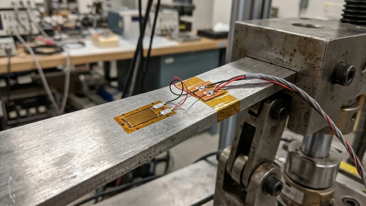
3. Stage 3 — Solder-Tab and Copper-Pad Notch Fracture: As TN-508-1 Appendix A emphasizes, most physical fatigue fractures in a strain gauge occur in the solder tab and the tab-to-outer-gridline transition area, not in the center of the active grid.

Why Copper-Coated Tabs (CEA) and Heavy Solder Fillets Cut Fatigue Life

General-purpose CEA-series gauges are popular for static stress analysis because they feature large, rugged, soft-copper-coated solder tabs encapsulated up to the tab boundary. However, in a dynamic cyclic strain field, those copper-coated tabs become a mechanical liability (TN-508-1, page 4):

• Copper and solder have lower fatigue endurance than Constantan or Karma foil: When an installer tins the entire CEA copper tab up to the polyimide encapsulation line, cyclic strain cracks the soft copper layer and the stiff solder fillet long before the Constantan (A-alloy) grid reaches its endurance limit.
• Mechanical notch propagation: Once a fatigue crack forms in the copper coating or at the stiff encapsulant/solder/copper boundary, it acts as a sharp mechanical stress-concentration notch directly bonded to the underlying foil, propagating the crack through the foil tab and severing the electrical circuit prematurely.

Gauge Tab & Lead Construction	Representative Catalog Series	Cyclic Fatigue Vulnerability	Recommended Dynamic Installation Practice (TN-508-1 Appendix A)
Large Copper-Coated Tabs	CEA Series	High notch risk if tinned across full tab; 10^5 cycles at ±1,500 με (10^6 at ±1,300 με)	Mask tab with PDT-1 drafting tape so solder is confined to a small dot in the bottom one-third of the tab; use low-modulus 50-50% Tin-Indium or 361A-20R (63-36.7-0.3% Pb-Sn-Sb) solder
Open-Face Foil Tabs	EA, EK (DP/DD duplex copper pads)	Moderate; unencapsulated grid is vulnerable to handling damage; Option LE pre-attached leads fail early in fatigue	Order Option E or Option SE encapsulation (EA); never use EA with Option LE in cyclic fatigue fields
Encapsulated with Controlled Solder Dots	SA, SK, SD, EA-Option SE	Low; factory solder dots restrict solder mass and prevent solder flow toward the grid transition (TT-606)	Attach fine jumper leads to the pre-formed solder dots (10^7 cycles at ±1,500 με on SA and ±2,000 με on SK)
Encapsulated with Pre-Attached Beryllium-Copper Leads	WK, WD, WA	Lowest; beryllium-copper ribbons have superior fatigue endurance and eliminate on-tab soldering heat (TT-604)	Highest cyclic endurance (10^7 cycles at ±2,200 με on WK and ±2,500 με on WD); land ribbons onto a bonded terminal strip

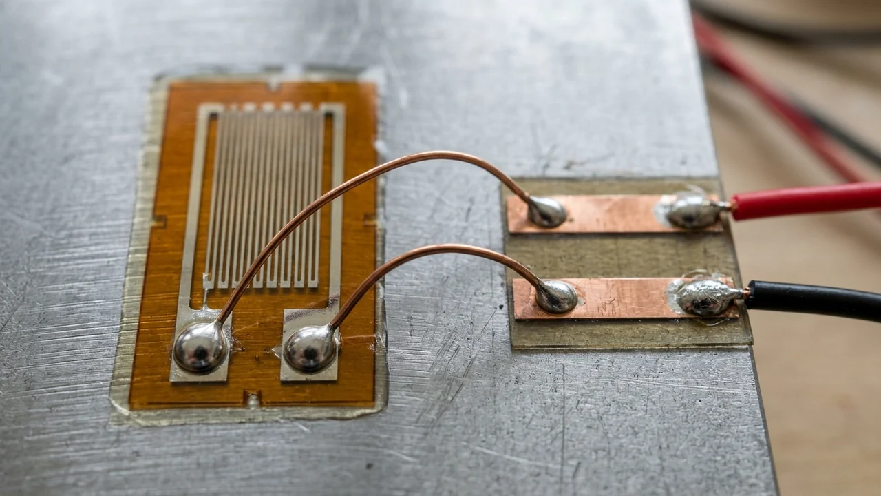
To achieve full catalog fatigue life on any dynamic strain gauge installation, enforce five physical rules from TN-508-1 Appendix A:

1. Orient solder tabs toward the lowest strain region: When the specimen’s strain gradient is known, orient the gauge so the solder tabs and tab-to-grid transitions sit in the lower-strain end of the footprint, and route jumper wires onto the tabs along the minimum-strain direction.
2. Interconnect via fine jumper wires and a bondable terminal strip (TT-603): Never solder heavy multi-strand instrument cables (22–26 AWG) directly to strain gauge tabs. Bond an intermediate terminal strip to the specimen (ideally in a lower-strain zone) and bridge from the terminal strip to the gauge tabs with small-diameter stress-relieved jumper wires.
3. Use flexible leadwire restraint, never rigid clamping, inside high-strain fields: Soft copper instrument leads fail in cyclic fatigue before the gauge grid if rigidly clamped to a flexing surface. Anchor the jumper leads as close as possible to the gauge backing with a flexible restraint—such as PDT-1 drafting tape, FA-2 aluminum foil tape, a small drop of M-Bond AE-10 epoxy, or M-Coat J polysulfide protective coating—to prevent tab peeling.
4. Select larger grid areas and moderate resistances (120 Ω or 350 Ω): Per TN-508-1 (page 1), larger active grid areas increase fatigue life, whereas miniature gauges (< 0.125 in [$3,\text{mm}$]) and ultra-thin high-resistance foils exhibit shorter fatigue life.
5. Remove excess edge adhesive: Scrape or wipe away thick beads of excess cement around the perimeter of the gauge carrier before curing; thick edge fillets crack under cyclic strain and propagate delamination into the gauge bond (TN-508-1, page 4).

Threshold rule: If your test requires $> 10^5$ load cycles above $\pm 1,300,\mu\varepsilon$ (or $> 2,340,\mu\varepsilon$ unidirectional peak-to-peak), do not tin the full copper tab of a CEA gauge or attach instrument cables directly to the gauge; switch to a WK, SK, WD, or SD series gauge (or mask CEA solder to the bottom $1/3$ of the tab with 50-50% Tin-Indium solder) and route fine jumper loops to a bonded intermediate terminal strip.

Takeaway: Monitor dynamic strain channels on an oscilloscope for tension-peak “super-sensitivity” distortion, and treat solder tabs, jumper loops, and terminal strips as fatigued structural components.

What Causes Zero Drift in Static and Long-Term Strain Measurements?

In a static load-hold test, a dead-weight structural calibration, or a multi-month civil/mechanical monitoring installation, cyclic foil cracking is absent. Instead, the measurement is governed by whether an unstrained 0.0 με baseline remains at 0.0 με across hours, weeks, or years. Four physical mechanisms drive static zero drift:

1. Temperature-Induced Apparent Strain (Thermal Output, TN-504-1)

As Vishay Micro-Measurements Tech Note TN-504-1 (Strain Gage Thermal Output and Gage Factor Variation with Temperature) states in Section 2.0, thermal output is potentially the largest error source in static strain measurement. When the temperature of a bonded strain gauge changes by $\Delta T$ without any mechanical stress applied to the part, two concurrent effects alter the gauge resistance $R_0$:

• The electrical resistivity of the metal foil changes with temperature according to its thermal coefficient of resistance $\beta_G$.
• The test specimen expands or contracts at its thermal expansion coefficient $\alpha_S$, while the foil grid expands at $\alpha_G$. Because the foil is bonded to the specimen, it is forced to deform by $(\alpha_S - \alpha_G)\Delta T$ in an equal-biaxial thermal strain field.

Per TN-504-1 Equation (1), the net unit resistance change due to thermal output is the algebraic sum of both effects:

(ΔR / R_0)_T/O = [ β_G + F_G × ((1 + K_t) / (1 - ν_0 × K_t)) × (α_S - α_G) ] × ΔT

Expressed as indicated apparent strain ε_T/O (dividing by instrument gauge factor setting F_I):
ε_T/O = (1 / F_I) × [ β_G + F_G × ((1 + K_t) / (1 - ν_0 × K_t)) × (α_S - α_G) ] × ΔT

where:

• $\beta_G$ = temperature coefficient of resistance of the grid conductor ($^\circ\text{C}^{-1}$ or $^\circ\text{F}^{-1}$)
• $F_G$ = uniaxial gauge factor of the strain gauge
• $K_t$ = transverse sensitivity of the strain gauge (accounting for biaxial thermal expansion vs. uniaxial calibration)
• $\nu_0 = 0.285$ = Poisson’s ratio of the standard calibration beam material (TN-504-1, page 1)
• $\alpha_S, \alpha_G$ = thermal expansion coefficients of the substrate and grid alloy ($\text{ppm}/^\circ\text{C}$ or $\text{ppm}/^\circ\text{F}$)

In Self-Temperature-Compensated (S-T-C) Constantan (A) and Modified Karma (K) foils, manufacturers cold-roll and heat-treat the alloy so that $\beta_G$ is negative or positive by just the right amount to cancel $F_G ((1 + K_t)/(1 - \nu_0 K_t))(\alpha_S - \alpha_G)$ near room temperature ($23^\circ\text{C}$ / $73^\circ\text{F}$) on a specific substrate material. Common S-T-C numbers (defined in $\text{ppm}/^\circ\text{F}$ in TN-505-4, page 2, and matched in $\text{ppm}/^\circ\text{C}$ in DwyerOmega Strain Gage Technical Data, page E-7) include:

• S-T-C 06 (~6.1 ppm/°F / 10.8–11 ppm/°C): Matched to ferritic carbon steel and martensitic stainless steels.
• S-T-C 09 (~9 ppm/°F / 16 ppm/°C): Matched to austenitic stainless steels (304/316) and copper alloys.
• S-T-C 13 (~12.8 ppm/°F / 23 ppm/°C): Matched to wrought aluminum alloys (2024, 6061, 7075).
• S-T-C 00 to 50: Available across 00, 03, 05, 06, 09, 13, 15, 18, 30, 40, 50 in A-alloy (for low-expansion quartz/graphite up to high-expansion plastics) and 00, 03, 05, 06, 09, 13, 15 in K-alloy.

Even with a matched S-T-C gauge, $\beta_G$ and $(\alpha_S - \alpha_G)$ vary nonlinearly with temperature, producing a polynomial thermal output curve over wide temperature swings. When ambient temperature varies during a static test, engineers either fit the lot’s polynomial thermal output curve using a bonded temperature sensor (ETG-50 / WTG-50 per TN-502 or an RTD/thermocouple) or wire an unstrained dummy compensating gauge on an identical block of substrate material into the adjacent Wheatstone bridge arm as detailed in our quarter, half, and full Wheatstone bridge guide. In a quarter-bridge hookup, leadwire resistance drift must also be canceled using a matched three-wire cable per our three-wire quarter-bridge checks guide.

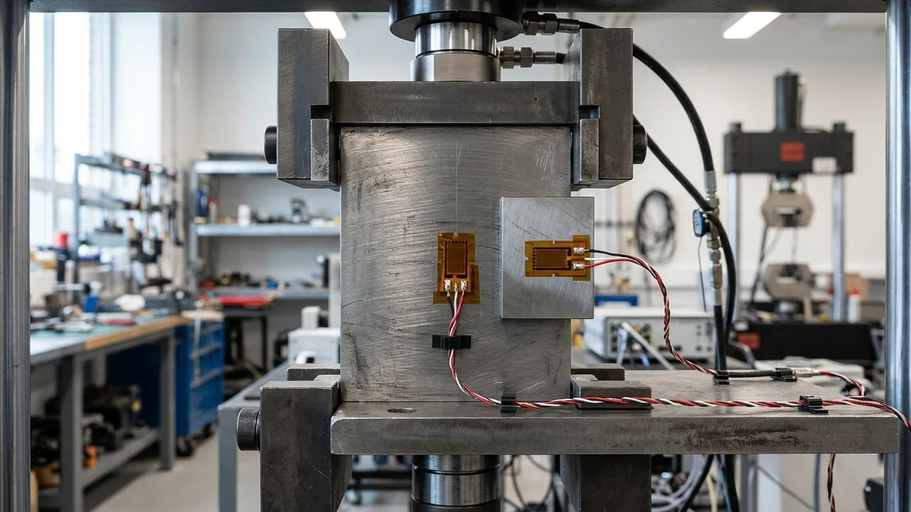
2. Constantan Alloy Drift Above +150°F (+65°C) vs. Modified Karma Stability

A critical specification trap in static testing is assuming that a Constantan (A-alloy) gauge can hold a stable zero reference anywhere inside its nominal operating temperature range (-75°C to +175°C on EA/CEA or -75°C to +200°C on SGD). Per Vishay TN-505-4 (Section 2.1.1, page 2), Constantan exhibits continuous metallurgical zero drift at temperatures above $+150^\circ\text{F}$ ($+65^\circ\text{C}$), which accumulates over hours or days.

For static strain measurements lasting months or years at room temperature, or static tests at elevated temperatures between $+65^\circ\text{C}$ and $+260^\circ\text{C}$ ($+500^\circ\text{F}$), TN-505-4 (Section 2.1.3, page 3) specifies Modified Karma (K-alloy, WK/SK/EK/S2K series) because Karma provides:

• Negligible metallurgical zero drift over multi-month and multi-year static holds.
• Extended static operating range from $-269^\circ\text{C}$ to $+260^\circ\text{C}$ ($-452^\circ\text{F}$ to $+500^\circ\text{F}$), and up to $+400^\circ\text{C}$ ($+750^\circ\text{F}$) short-term when encapsulated.
• A significantly flatter thermal output curve across temperature extremes than Constantan.

3. Adhesive Creep and Glueline Thickness (0.0025–0.0075 mm)

The adhesive layer and polymer carrier sit physically in series between the specimen surface and the metallic foil grid, acting as a mechanical spring that transmits shear force into the grid (A05, page E-3). If the adhesive undergoes viscoelastic relaxation under sustained load, the foil grid relaxes backward and reports a decaying strain (creep).

• Short-term room-temperature tests (< 10^4 hours, -45°C to +65°C): Cyanoacrylate (M-Bond 200) or two-part room-temperature curing epoxy (M-Bond AE-10) is acceptable for moderate-accuracy stress analysis (TN-505-4 Selection Chart, page 5).
• Long-term static stability (> 10^4 hours), high accuracy, or elevated temperature (up to +230°C / +370°C): Require heat-cured, unfilled, thin-film-setting epoxies (M-Bond AE-15, M-Bond 600, or M-Bond 610).
• Ideal glueline thickness (TN-502, page 1): Do not use adhesives loaded with aluminum-oxide or metal-powder thermal fillers; fillers raise viscosity and create a thick glueline that increases both mechanical creep and thermal resistance. On smooth mounting surfaces, clamp the gauge during cure to achieve an unfilled glueline thickness of $0.0001$ to $0.0003,\text{in}$ ($0.0025$ to $0.0075,\text{mm}$).

4. Surface Contamination and Insulation Resistance (≥ 500 MΩ)

Before zeroing any static strain channel, measure the DC insulation resistance between the strain gauge leadwires and the conductive metal specimen using a low-voltage megohmmeter or high-impedance ohmmeter (never a high-voltage insulation tester that would burn out the foil grid). Per DwyerOmega Strain Gage Technical Data (page E-3), an insulation resistance below $500,\text{M}\Omega$ indicates surface flux contamination, incomplete solvent cleaning, or moisture ingress. A $100,\text{M}\Omega$ leakage path in parallel with a $350,\Omega$ bridge arm acts as an unstable parasitic shunt resistor that drifts with ambient relative humidity, masquerading as mechanical creep.

Takeaway: For static holds exceeding a few hours or operating above $+65^\circ\text{C}$ ($+150^\circ\text{F}$), replace Constantan (CEA/EA) and cyanoacrylate (M-Bond 200) with Modified Karma (WK/SK/EK) bonded using a $0.0025\text{–}0.0075,\text{mm}$ thin-film epoxy (M-Bond AE-15/600/610), and verify $\ge 500,\text{M}\Omega$ insulation resistance to ground.

How Do Alloy, Backing, and Excitation Power Density Specifications Pair Together?

Because every commercial strain gauge series is manufactured as an integrated foil-and-backing system (TN-505-4, Section 2.2), choosing a gauge requires matching the test profile (static vs. dynamic, temperature, strain level, and duration) to both the catalog series and the allowable bridge excitation power density.

Vishay TN-505-4 Series & Adhesive Selection Matrix by Test Profile

Test Regime & Operating Temperature	Duration / Cycle Requirement	Peak Strain (με)	Accuracy Class	Recommended Vishay Series (TN-505-4, p. 5)	Recommended M-Bond Adhesive
General Static or Static-Dynamic (-45°C to +65°C / -50°F to +150°F)	< 10^4 hours, < 10^6 cycles	±1,300 με	Moderate	CEA, EA (or Omega SGD / KFG)	200 or AE-10
Extended Static or Static-Dynamic (-45°C to +65°C / -50°F to +150°F)	> 10^4 hours, < 10^6 cycles	±1,300 με	Moderate	CEA, EA	AE-10 or AE-15
High-Accuracy Long-Term Static / Dynamic (-45°C to +65°C)	> 10^4 hours, > 10^6 cycles	±1,600 με / ±2,000 με	Very High	WA, SA (±1,600 με) or WK, SK (±2,000 με)	AE-15 or 610
Elevated-Temp Static or Static-Dynamic (-45°C to +205°C / -269°C to +230°C)	> 10^3 to > 10^4 hours, < 10^6 to > 10^6 cycles	±1,600 με to ±2,000 με	Moderate to High	WA, SA (±1,600 με) or WK, SK (±2,000 με)	600 or 610
High-Elongation Post-Yield Static (-45°C to +65°C)	Single monotonic excursion (N = 1)	±50,000 με (±5%)	Moderate	CEA, EA	AE-10
Extreme Post-Yield Plastic Static (-45°C to +65°C)	Single monotonic excursion (N = 1)	±100,000 με (10%) / ±200,000 με (20%)	Moderate	EP (Annealed Constantan)	AE-15 (10%) or A-12 (20%)
Purely Dynamic High-Cycle Fatigue (-195°C to +205°C / +260°C)	10^6 to 10^8 cycles (AC-coupled, no DC zero required)	±2,200 με to ±3,000 με	Dynamic SNR Priority	ED, SD, WD (Isoelastic, GF ≈ 3.2) or WK	AE-15, 600, or 610

Static vs. Dynamic Bridge Excitation Power Density (TN-502 Table 1)

In an equal-arm Wheatstone bridge excited by voltage $E_B$, the electrical power dissipated as heat inside a single strain gauge grid of resistance $R_G$ and active grid area $A_G = L_{\text{grid}} \times W_{\text{grid}}$ is given by Vishay Micro-Measurements Tech Note TN-502 (Optimizing Strain Gage Excitation Levels) (page 3):

Power dissipated in grid (W):
  P_G = E_B^2 / (4 × R_G)

Grid power density (W/in² or kW/m², where 1 W/in² = 1.55 kW/m²):
  P'_G = P_G / A_G = E_B^2 / (4 × R_G × A_G)

Maximum allowable bridge excitation voltage E_B for target power density P'_G:
  E_B = 2 × sqrt(R_G × P'_G × A_G)

Because localized Joule heating raises the grid temperature above the specimen surface temperature, excessive excitation causes three static errors (TN-502, page 1): (1) loss of Self-Temperature-Compensation (S-T-C curves are calibrated at near-zero self-heating), (2) accelerated backing and glueline creep, and (3) zero-stability drift whenever slight heat-sink differences exist between bridge arms.

Crucially, TN-502 (Section 5, page 2) notes that self-heating degrades static zero stability far more severely than dynamic AC response. In a purely dynamic test where slow thermal baseline shifts are rejected, you can drive the bridge at $2.5\times$ to $5\times$ higher power density $P’_G$—increasing bridge excitation voltage $E_B$ by $\sqrt{2.5} \approx 1.58\times$ to $\sqrt{5} \approx 2.24\times$ and directly boosting dynamic signal-to-noise ratio:

Substrate Heat-Sink Class & Specimen Examples (TN-502 Table 1)	Static: High Accuracy (W/in² [kW/m²])	Static: Moderate Accuracy (W/in² [kW/m²])	Static: Low Accuracy (W/in² [kW/m²])	Dynamic: High Accuracy (W/in² [kW/m²])	Dynamic: Moderate Accuracy (W/in² [kW/m²])	Dynamic: Low Accuracy (W/in² [kW/m²])
Excellent: Heavy Aluminum or Copper Specimen	2–5 [3.1–7.8]	5–10 [7.8–16]	10–20 [16–31]	5–10 [7.8–16]	10–20 [16–31]	20–50 [31–78]
Good: Thick Structural Steel Specimen	1–2 [1.6–3.1]	2–5 [3.1–7.8]	5–10 [7.8–16]	5–10 [7.8–16]	10–20 [16–31]	20–50 [31–78]
Fair: Thin Stainless Steel or Titanium	0.5–1 [0.78–1.6]	1–2 [1.6–3.1]	2–5 [3.1–7.8]	2–5 [3.1–7.8]	5–10 [7.8–16]	10–20 [16–31]
Poor: Filled Plastic (Fiberglass / Epoxy FRP)	0.1–0.2 [0.16–0.31]	0.2–0.5 [0.31–0.78]	0.5–1 [0.78–1.6]	0.5–1 [0.78–1.6]	1–2 [1.6–3.1]	2–5 [3.1–7.8]
Very Poor: Unfilled Plastic (Acrylic, Polystyrene)	0.01–0.02 [0.016–0.031]	0.02–0.05 [0.031–0.078]	0.05–0.1 [0.078–0.16]	0.01–0.05 [0.016–0.078]	0.05–0.2 [0.078–0.31]	0.2–0.5 [0.31–0.78]

Stacked Rosette Derating Rule (TN-502, page 2): When using a superimposed strain gauge rosette for principal strain orientation, heat from the bottom grids flows through the upper grids. In a 3-element stacked rosette, the top grid experiences $6\times$ the temperature rise of a single unstacked grid at the same power; reduce per-grid power to $1/6$ by dividing allowable single-grid bridge excitation voltage $E_B$ by $2.5$. In a 2-element stacked rosette, reduce per-grid power to $1/3$ by dividing $E_B$ by $1.7$.

Worked Example 2: Static vs. Dynamic Excitation Voltage and Series Dropping Resistor (TN-502 Cases 1 & 2)

Suppose you bond an EA-09-125AD-120 strain gauge ($R_G = 120,\Omega$, active grid area $A_G = 0.125,\text{in} \times 0.125,\text{in} = 0.0156,\text{in}^2$ [$10.06,\text{mm}^2$]) to a thin $1/2 \times 1/16 \times 6,\text{in}$ ($12.5 \times 1.5 \times 150,\text{mm}$) stainless-steel bar (“Fair” heat-sink class):

1. Allowable Bridge Excitation for Static Moderate Accuracy (P'_G = 1 to 2 W/in² per TN-502 Case 1):
   • At P'_G = 1.0 W/in² (1.6 kW/m²):
     E_B_min = 2 × sqrt(120 Ω × 1.0 W/in² × 0.0156 in²) = 2 × sqrt(1.872) = 2.74 V (≈ 2.7 V)
   • At P'_G = 2.0 W/in² (3.1 kW/m²):
     E_B_max = 2 × sqrt(120 Ω × 2.0 W/in² × 0.0156 in²) = 2 × sqrt(3.744) = 3.87 V (≈ 3.8 V)
   => Safe static bridge excitation range is 2.7 V to 3.8 V maximum.

2. Contrast with Purely Dynamic Moderate Accuracy on the Same Bar (P'_G = 5 to 10 W/in²):
   • At P'_G = 5.0 W/in²:
     E_B_dyn_min = 2 × sqrt(120 Ω × 5.0 W/in² × 0.0156 in²) = 2 × sqrt(9.36) = 6.12 V
   • At P'_G = 10.0 W/in²:
     E_B_dyn_max = 2 × sqrt(120 Ω × 10.0 W/in² × 0.0156 in²) = 2 × sqrt(18.72) = 8.65 V
   => Dynamic AC testing allows up to 6.1–8.6 V on the same 120 Ω gauge, more than doubling signal output.

3. Series Dropping Resistor R_D when Using a Fixed 4.5 V Static Indicator (TN-502 Case 2):
   • At a fixed E_B = 4.5 V, actual grid power density is:
     P'_G = (4.5 V)^2 / (4 × 120 Ω × 0.0156 in²) = 20.25 / 7.488 = 2.70 W/in² (4.2 kW/m²)
     which exceeds the 2.0 W/in² static limit.
   • Insert an inactive precision series resistor R_D in both the active and dummy arms:
     R_D = (E_B / 2) × sqrt(R_G / (A_G × P'_G_desired)) - R_G
         = (4.5 / 2) × sqrt(120 / (0.0156 × 2.0)) - 120
         = 2.25 × sqrt(3,846.15) - 120 = 139.54 - 120 = 19.5 Ω
   • Correct indicated static strain readings for the series desensitization factor:
     Correction Multiplier = (R_D + R_G) / R_G = (19.5 + 120) / 120 = 1.1625 (≈ 1.16×)

Notice the resistance trade-off between static self-heating and dynamic fatigue: switching from $120,\Omega$ to $350,\Omega$ or $1,000,\Omega$ reduces grid heating power $P_G = E_B^2 / (4 R_G)$ by $2.9\times$ or $8.3\times$ at a given voltage (TN-502; A07), which is ideal for static stability and composite substrates. However, for small grid footprints in severe cyclic fatigue fields, TN-508-1 (page 1) warns that very high resistance gauges etched from ultra-thin foil have lower cyclic fatigue life than standard $120,\Omega$ or $350,\Omega$ grids of sufficient area ($L \ge 0.25,\text{in}$ [$6.4,\text{mm}$]).

Takeaway: Size bridge excitation voltage from $E_B = 2\sqrt{R_G P’_G A_G}$ using the static vs. dynamic rows of TN-502 Table 1, and choose $350,\Omega$ grids of $\ge 0.125\text{–}0.25,\text{in}$ ($3.2\text{–}6.4,\text{mm}$) length when balancing static thermal dissipation against cyclic fatigue life.

Installation Scope Drivers and Pre-Test Specification Checklist

As Vishay TN-505-4 (Section 1.0, page 1) emphasizes, the purchase price of the strain gauge foil itself is a small fraction of the total cost of an instrumented test channel. Rework, fixture downtime, and invalidated test runs are driven by five scope factors:

1. Adhesive cure schedule and clamping fixtures: Switching from cyanoacrylate (M-Bond 200, 1-minute thumb pressure at room temperature) to high-stability/high-fatigue thermosetting epoxy (M-Bond AE-15 or M-Bond 600/610) requires spring-loaded clamping pads ($30\text{–}50,\text{psi}$) and elevated-temperature oven or heat-lamp curing plus post-cure thermal cycling.
2. Leadwire strain relief and intermediate terminal bonding (TT-603 / TT-604): Dynamic cyclic channels require bonding separate two- or three-tab terminal strips, forming stress-relieved jumper loops, masking copper tabs or ordering pre-leaded WK/WD gauges, and applying flexible elastomeric coatings (M-Coat J).
3. Thermal compensation hardware: Static channels exposed to ambient temperature swings require bonding either an unloaded dummy gauge on a matching substrate block (Quarter-Bridge Type II) or a bondable resistance temperature sensor (ETG-50/WTG-50) on an extra DAQ channel.
4. Channel bandwidth and sample-rate storage: Static stepwise load tests log at $1\text{–}100,\text{S/s}$ on portable bridge indicators (P3/D4), whereas dynamic cyclic and transient impact tests require $1,\text{kS/s}$ to $10,\text{MS/s}$ simultaneous digitizers (A04, page 1; see our DAQ sample rate planning worksheet and strain gauge amplifier bandwidth guide).
5. Packaged transducer alternative: When the engineering goal is measuring net structural force or weight rather than localized surface stress, bonding and calibrating bare field gauges is often more labor-intensive than mounting a factory-compensated full-bridge load cell (see our strain gauge vs load cell comparison) or a reusable bolt-on piezoresistive dynamic strain transducer.

Six-Point Pre-Acquisition Verification Sequence

Before starting a static load hold or a dynamic fatigue run, verify and log these six checks on each installed channel:

1. Check peak strain against both monotonic and cyclic limits: Confirm that monotonic peak strain stays within the carrier’s static rating ($\pm 15,000,\mu\varepsilon$ for W-backing, $\pm 30,000\text{–}50,000,\mu\varepsilon$ for EA/CEA/SGD, $\pm 200,000,\mu\varepsilon$ for EP) and that cyclic peak-to-peak strain converted via $|\varepsilon_{\text{rev}}| = \Delta\varepsilon_{\text{p-p}} / 1.80$ falls below the TN-508-1 $100,\mu\varepsilon$ zero-shift curve for your target cycle count $N$.
2. Verify S-T-C number and alloy temperature ceiling: Match the gauge S-T-C code (06 for ferritic steel, 13 for aluminum) to the specimen material, and confirm Constantan (A-alloy) is not used for static zero-stability holds above $+65^\circ\text{C}$ ($+150^\circ\text{F}$).
3. Measure unstrained grid resistance $R_G$ and ground insulation resistance ($\ge 500,\text{M}\Omega$): Check series loop continuity against package nominal resistance ($120,\Omega$, $350,\Omega$, or $1,000,\Omega \pm \text{tolerance}$) and verify $\ge 500,\text{M}\Omega$ insulation between grid leads and the metal structure (A05, page E-3).
4. Inspect glueline edges, solder-tab masking, and jumper strain relief: Confirm excess perimeter adhesive has been removed, solder occupies only the outer third of CEA tabs (or factory solder dots / BeCu ribbons), and fine jumper wires arc into a bonded terminal strip along the minimum-strain direction (TN-508-1, page 4).
5. Verify bridge excitation voltage $E_B$ at zero load (TN-502 test): Compute $P’_G = E_B^2 / (4 R_G A_G)$ (applying the $2.5\times$ or $1.7\times$ voltage reduction for 3-grid or 2-grid stacked rosettes) and confirm the unloaded zero reading remains stable when switching from low excitation to operating excitation (TN-502, page 3).
6. Monitor cyclic waveform symmetry on an oscilloscope (TN-508-1 test): During dynamic fatigue testing, inspect the live time-domain waveform periodically for upward tensile-peak distortion (“super-sensitivity”) or a diverging tensile-versus-compressive amplitude ratio that signals incipient foil micro-cracking.

Three-Parameter Engineering Specification Worksheet

Before selecting a strain gauge catalog series, adhesive, and DAQ conditioner mode, define these three test parameters for your channel record:

Parameter to Define	Engineering Input Required	How It Governs Your Gauge & DAQ Selection
1. Loading Regime & Target Cycle Count (N)	Is the load a static sustained hold / stepwise FEA check (N = 1), a combined static-dynamic load, or an alternating cyclic / impact load (specify target cycles $N = 10^4, 10^5, 10^6, 10^7,$ or $10^8$)?	Determines whether monotonic elongation (CEA/EA/EP), combined zero-stability + fatigue (WK/SK), or purely dynamic AC fatigue (WD/SD) governs.
2. Estimated Peak Microstrain (με)	What is the maximum monotonic strain ($\mu\varepsilon$) and the alternating peak-to-peak cyclic strain excursion $\Delta\varepsilon_{\text{p-p}} = \varepsilon_{\text{max}} - \varepsilon_{\text{min}}$ ($\mu\varepsilon$)?	Sets the equivalent fully reversed cyclic strain $
3. Test Duration, Thermal Span & Coupling Mode	How long must the test hold a zero reference (seconds/minutes vs. hours/months/years), what is the ambient temperature range ($^\circ\text{C}$), and does the DAQ channel require DC coupling or AC coupling?	Selects the alloy/adhesive (M-Bond 200 vs. AE-15/610; Constantan < +65°C vs. Karma up to +260°C), S-T-C / dummy-bridge compensation, and TN-502 static vs. dynamic excitation power density $P’_G$.

Takeaway: Lock down the loading regime and target cycle count $N$, peak-to-peak microstrain excursion $\Delta\varepsilon_{\text{p-p}}$, and required zero-stability duration before ordering gauges or setting bridge excitation voltage.

Technical References and Sources

All specification thresholds, fatigue life curves, thermal output equations, and excitation power-density limits in this guide are compiled from the following primary technical notes and manufacturer reference documents (reviewed 27 October 2026):

1. Vishay Micro-Measurements Tech Note TN-508-1: Fatigue Characteristics of Micro-Measurements Strain Gages — Defines cyclic zero-shift ($100,\mu\varepsilon$ standard criterion; $300,\mu\varepsilon$ for WD series), tensile super-sensitivity waveform distortion, Table 1 nominal fatigue life across CEA, EA, EP, WA, SA, EK, S2K, WK, SK, ED, SD, and WD series on $0.25,\text{in}$ ($6.4,\text{mm}$) gauges, the $10%$ peak-to-peak unidirectional derating rule, and Appendix A installation practices.
2. Vishay Micro-Measurements Tech Note TN-505-4: Strain Gage Selection: Criteria, Procedures, Recommendations — Specifies sensing alloys (A Constantan, P Annealed Constantan, D Isoelastic, K Modified Karma), carrier backings (E polyimide vs. W/S glass-fiber-reinforced epoxy-phenolic), Self-Temperature-Compensation (S-T-C) numbers, static elongation ratings vs. cyclic endurance, and M-Bond adhesive pairings.
3. Vishay Micro-Measurements Tech Note TN-504-1: Strain Gage Thermal Output and Gage Factor Variation with Temperature — Derives Equation (1) for temperature-induced apparent strain $(\Delta R / R_0)_{T/O}$ and transverse-sensitivity biaxial thermal correction.
4. Vishay Micro-Measurements Tech Note TN-502: Optimizing Strain Gage Excitation Levels — Establishes grid power dissipation $P_G = E_B^2 / (4 R_G)$, ideal unfilled glueline thickness ($0.0001\text{–}0.0003,\text{in}$ [$0.0025\text{–}0.0075,\text{mm}$]), stacked rosette derating ($1/6$ power / $2.5\times$ voltage reduction for 3-grid stacked rosettes), Case 1 and Case 2 worked examples, and Table 1 allowable power-density limits ($\text{W/in}^2$ and $\text{kW/m}^2$) for static vs. dynamic measurements.
5. Vishay Micro-Measurements StrainBlog (11 October 2023): Static vs. Dynamic Strain Gage Testing — Contrasts stepwise static load-hold testing and FEA validation against dynamic cyclic and transient impact testing ($1,\text{kS/s}$ to $10,\text{MS/s}$ sampling rates and field leadwire protection).
6. DwyerOmega Technical Reference (Pages E-3 to E-10): Strain Gage Technical Data — Provides side-by-side SGD and KFG series specifications at $23^\circ\text{C}$ ($73^\circ\text{F}$) reference temperature, including $3%$ ($30,000,\mu\varepsilon$) maximum static strain vs. $>10^7$ cycles at $\pm 1,500,\mu\varepsilon$ fatigue life and the $\ge 500,\text{M}\Omega$ post-installation insulation resistance threshold.
7. National Instruments Sensor Fundamentals (Updated 2026): Measuring Strain with Strain Gages — Details nominal gauge resistances ($120,\Omega$, $350,\Omega$, $1,000,\Omega$), grid width trade-offs, and quarter-, half-, and full-bridge sensitivity and temperature compensation configurations.