Strain Gauge Amplifier and Signal Conditioning: Gain, Excitation, and Bandwidth

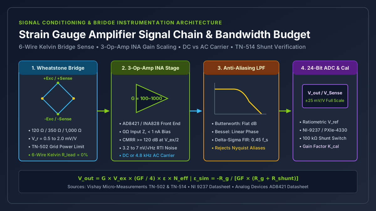
A strain gauge amplifier conditions the microvolt-to-millivolt differential output of a Wheatstone bridge to match the full-scale input span of an analog-to-digital converter while rejecting the half-excitation common-mode voltage pedestal and regulating bridge excitation power. Selecting excessive excitation voltage or omitting six-wire Kelvin sense and shunt calibration causes localized grid self-heating drift, uncompensated cable span attenuation exceeding 1.4% on 30 m runs, and out-of-band aliasing that corrupts peak structural force measurements.

Size a strain gauge signal conditioning chain in four sequential steps: bound the bridge excitation voltage V_ex using Vishay Tech Note TN-502 grid power density limits (P'_G = V_ex^2 / (4 × R_g × A_grid)), set the 3-op-amp instrumentation amplifier gain G = V_ADC_FS / (V_ex × V_r_FS) or ratiometric mV/V range with at least 120 dB common-mode rejection, select six-wire Kelvin remote sensing or three-wire quarter-bridge completion to cancel copper leadwire thermal drift, and verify end-to-end span scaling with a precision parallel shunt calibration resistor (ε_sim = -R_g / [GF × (R_g + R_shunt)]) per Vishay Tech Note TN-514.

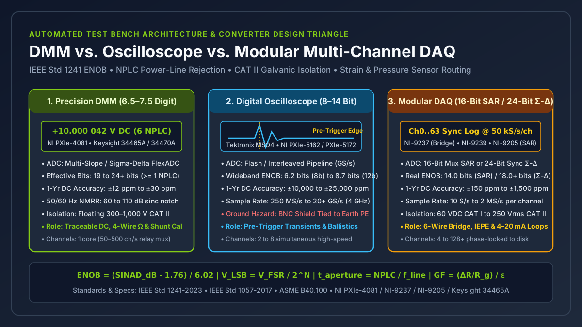
This engineering guide belongs to the Sensors and DAQ documentation hub, supports our strain gauge vs load cell comparison, and pairs with our DMM vs oscilloscope vs DAQ test bench architecture guide by detailing the analog front-end equations, excitation budgets, and filter topologies required once the sensor type is selected. Maximizing Value at NI is an independent technical publication (about this site) not affiliated with National Instruments (NI) or Emerson.

Signal Conditioner Architecture	Usable Signal Bandwidth (f_-3dB)	Typical CMRR (at G >= 100)	1/f Flicker & Thermocouple EMF Rejection	Typical Bridge Excitation	Primary Engineering Application
Wideband Bipolar/JFET 3-Op-Amp INA (AD8421, INA828)	0 Hz (DC) to 100 kHz – 2 MHz	120 dB to 140 dB (DC to 60 Hz)	Moderate (1/f corner at 10–100 Hz; sensitive to 0 Hz Seebeck EMF)	0.5 V to 10.0 V DC	High-speed impact, crash sleds, ballistic pressure, and shock transients
Chopper-Stabilized / Auto-Zero DC Bridge Conditioner	0 Hz (DC) to 1 kHz – 10 kHz	120 dB to 140 dB	High for amplifier 1/f drift (< 50 nV/°C); still passes sensor-side DC thermal EMF	1.0 V to 10.0 V DC	Static structural stress testing and multi-day lab creep logging
AC Carrier Synchronous Lock-In Amplifier (1.2–4.8 kHz)	0 Hz (DC) to 120 Hz – 1.0 kHz (<= 0.2 × f_carrier)	120 dB to 140 dB	Immune (blocks 0 Hz thermocouple EMF, 1/f noise, and 50/60 Hz magnetic hum)	1.0 V to 10.0 V RMS AC (600 Hz to 4.8 kHz)	Precision load cell weighing and fatigue rigs near 480 V VFD motors or furnaces
24-Bit Simultaneous Ratiometric Delta-Sigma Module (NI-9237, PXIe-4330)	0 Hz (DC) to 22.5 kHz (0.45 × f_s at 50 kS/s)	140 dB (at 0–60 Hz, ratiometric ±25 mV/V span)	High via ratiometric V_ref = (+Sense - -Sense) and optional digital offset nulling	2.5 V to 10.0 V DC (150 mW max total power on NI-9237)	Simultaneous multi-channel structural test rigs and rosette DAQ systems

Takeaway: Match the conditioner architecture to your upper frequency limit and electromagnetic environment first; wide bandwidth requires DC excitation, whereas immunity to thermocouple offsets and 60 Hz motor hum favors AC carrier demodulation.

How Do Strain Gauge and Gauge Factor Equations Set Bridge Millivolt Levels?

Designing or configuring a strain gauge amplifier begins with the electromechanical transfer function of the sensing grid. Mechanical strain ε is defined as the fractional change in length ε = ΔL / L (dimensionless, typically expressed in microstrain με = ε × 10^6, where 1,000 με equals a 0.10% length change or 10^-3 m/m). For foundational derivations of grid geometry and transverse sensitivity, see our strain gauge basics and gauge factor explainer.

The relationship between a strain gauge and gauge factor (GF or F_G) links mechanical deformation to fractional resistance change:

GF = (ΔR / R_g) / ε     =>     ΔR = R_g × GF × ε

where R_g is the unstrained nominal gauge resistance in ohms (120 Ω, 350 Ω, or 1,000 Ω) and ΔR is the strain-induced resistance change in ohms. On a standard 350 Ω metallic foil grid with GF = 2.00 subjected to +1,000 με tensile strain, the fractional resistance shift is ΔR / R_g = 2.00 × 10^-3 = 0.20%, which equals a resistance change of only +0.70 Ω (raising total arm resistance from 350.00 Ω to 350.70 Ω). On a 120 Ω grid at +1,000 με, ΔR is only +0.24 Ω.

Sensing Grid Alloy / Material	Typical Gauge Factor (GF)	Temperature & Fatigue Behavior	Typical Bridge Conditioning Target
Constantan (A-alloy, 55% Cu / 45% Ni foil)	2.00 to 2.10 (nominal 2.05 ± 1%)	Self-temperature-compensated (STC 06 for steel ~10.8 ppm/°C, STC 13 for aluminum ~23 ppm/°C); wide linear strain range (±3% to ±5%)	Quarter-, half-, and full-bridge experimental stress analysis (0.5 to 2.0 mV/V per 1,000 με)
Modified Karma (K-alloy, Ni-Cr foil)	2.05 to 2.15 (nominal 2.10)	Superior fatigue life, low creep, and flat thermal output from -75°C to +200°C	Calibrated strain gauge force sensor spring elements (S-beam, shear-web, and canister load cells)
Isoelastic (D-alloy, Fe-Ni-Cr-Mo foil)	3.20 to 3.50	60% higher output and long cyclic fatigue life, but high temperature coefficient of resistance prohibits static DC measurement	AC-coupled dynamic vibration and rotating shaft impact strain
Monocrystalline Silicon (P-type / N-type semiconductor)	+100 to +175 (P-type) or -100 to -150 (N-type)	50× to 75× higher sensitivity for sub-microstrain (< 0.1 με) resolution, but strong TCR (~0.15%/°C), TCGF (~-0.2%/°C), and nonlinearity	High-stiffness miniature force sensors and MEMS pressure diaphragms

Because measuring a 0.24 Ω change directly on top of a 120 Ω baseline requires resolving 2,000 ppm full scale (and 0.2 ppm per 0.1 με), strain gauges are wired into a Wheatstone bridge excited by a stabilized voltage V_ex. As derived in our quarter, half, and full Wheatstone bridge comparison and National Instruments’ SCXI-1520 User Manual (Chapter 4), the small-strain linear bridge output ratio V_r (in V/V or mV/V) is:

V_r = V_out / V_ex = (GF / 4) × ε × N_eff
V_out = V_ex × (GF / 4) × ε × N_eff

where N_eff is the effective number of additive active arms:

1. Quarter-bridge (N_eff = 1): One active gauge and three passive completion resistors. At GF = 2.00, sensitivity is 0.50 μV/V per με (0.50 mV/V at 1,000 με). With V_ex = 5.0 V, a 1,000 με load produces 2.50 mV differential signal riding on a +2.50 V common-mode pedestal (V_ex / 2). Using the exact nonlinear bridge equation V_r = (GF × ε) / [4 × (1 + (GF × ε) / 2)], the output at 1,000 με is 0.4995 mV/V (0.10% bridge nonlinearity, reaching 1.0% at 10,000 με).
2. Half-bridge axial Poisson (N_eff = 1 + ν) or bending (N_eff = 2): A bending half bridge with opposite-face tensile and compressive grids yields 1.00 μV/V per με (5.00 mV at 1,000 με and V_ex = 5.0 V), while an axial + Poisson half bridge on steel (ν = 0.30) yields 0.65 μV/V per με (3.25 mV at 1,000 με).
3. Full-bridge strain gauge force sensor (N_eff = 4 for bending/shear web, or 2 × (1 + ν) for axial column): Commercial load cells and reaction torque transducers bond four matched Karma or Constantan grids onto a machined alloy steel, stainless steel, or aluminum spring element configured so that rated mechanical force produces roughly 1,000 με to 1,500 με surface strain. At GF = 2.00 and N_eff = 4, 1,000 με generates a rated transducer output of 2.00 mV/V (10.00 mV full-scale output at V_ex = 5.0 V, or 20.00 mV at V_ex = 10.0 V).

Takeaway: Whether you bond a single quarter-bridge foil grid (0.5 mV/V at 1,000 με) or wire a calibrated 2.0 mV/V full-bridge strain gauge force sensor, the conditioner must extract microvolt-level differential changes sitting on top of a multi-volt common-mode pedestal.

How Do You Size Instrumentation Amplifier Gain, CMRR, and Bridge Excitation Power?

A standard single-op-amp differential subtractor circuit cannot condition a Wheatstone bridge directly. Achieving low thermal Johnson noise in a four-resistor op-amp difference stage requires low-value input resistors (1 kΩ to 10 kΩ), which load the 120 Ω or 350 Ω bridge midpoints (+Sig and -Sig), corrupt bridge linearity, and degrade common-mode rejection unless resistor ratios match to better than 0.001%.

Instead, a dedicated strain gauge amplifier uses a three-op-amp instrumentation amplifier (INA) front end, such as the Analog Devices AD8421 (3.2 nV/√Hz input voltage noise, 2 MHz bandwidth at G = 100) or Texas Instruments INA828 (7.0 nV/√Hz input noise, 50 μV maximum offset). Two matched non-inverting input buffer amplifiers (A1 and A2) present gigohm input impedance (> 1 GΩ) and sub-nanoamp bias current to the bridge midpoints, followed by an integrated laser-trimmed difference amplifier (A3) that strips the V_ex / 2 common-mode pedestal. For grounding and bias-return checks on differential inputs, see our floating DAQ input wiring guide.

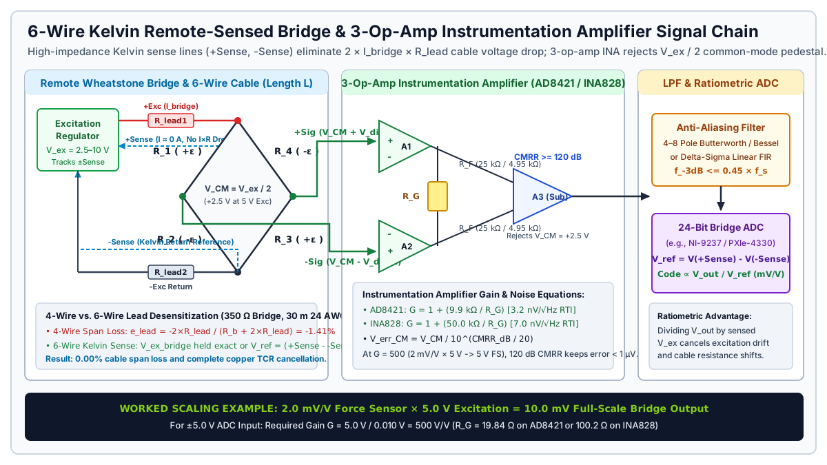
Worked Example 1: Gain Resistor and Noise Floor Sizing for a 2.0 mV/V Force Sensor

Suppose you are conditioning a 2.0 mV/V full-bridge strain gauge force sensor (350 Ω bridge resistance) with a regulated V_ex = 5.0 V DC supply into an analog-to-digital converter with a ±5.0 V full-scale input span (V_ADC_FS = 5.0 V), and you need to resolve 0.05% of full scale over a 100 Hz low-pass filter bandwidth:

1. Full-scale bridge differential voltage:
   V_bridge_FS = V_ex × V_r_FS = 5.0 V × 2.0 mV/V = 10.0 mV (0.010 V)

2. Required instrumentation amplifier voltage gain:
   G = V_ADC_FS / V_bridge_FS = 5.0 V / 0.010 V = 500 V/V (53.98 dB)
   (For a ±10.0 V ADC input range, G = 10.0 V / 0.010 V = 1,000 V/V = 60.0 dB)

3. Gain-setting resistor R_G selection:
   • Analog Devices AD8421: G = 1 + (9.9 kΩ / R_G)
     R_G = 9,900 Ω / (500 - 1) = 19.84 Ω
   • Texas Instruments INA828: G = 1 + (50.0 kΩ / R_G)
     R_G = 50,000 Ω / (500 - 1) = 100.20 Ω

4. Input-referred (RTI) thermal and amplifier noise check at T = 300 K:
   • 350 Ω bridge Johnson thermal noise density:
     e_n_bridge = sqrt(4 × k_B × T × R_g) = sqrt(4 × 1.38e-23 × 300 × 350) = 2.41 nV/√Hz
   • Total RTI voltage noise density with AD8421 (e_n_INA = 3.2 nV/√Hz):
     e_n_total = sqrt(3.2^2 + 2.41^2) = 4.01 nV/√Hz
   • Over a 4-pole Butterworth filter with f_-3dB = 100 Hz (ENBW ≈ 1.026 × 100 Hz = 102.6 Hz):
     V_noise_RMS_RTI = 4.01 nV/√Hz × sqrt(102.6 Hz) = 40.6 nV RMS (≈ 0.27 μV peak-to-peak)
   • Signal-to-noise ratio at 10.0 mV full scale:
     Dynamic range = 10,000 μV / 0.27 μV_pp ≈ 37,000:1 (91.4 dB peak-to-peak free resolution)

Common-Mode Rejection Ratio (CMRR) Requirements

When a bridge is powered by a single-ended +5.0 V or +10.0 V supply referenced to analog ground, both signal midpoints sit at a DC common-mode voltage V_CM = V_ex / 2 (+2.5 V or +5.0 V), plus any 50/60 Hz AC power-line interference capacitively coupled into the sensor shield. An amplifier with common-mode rejection ratio CMRR_dB converts common-mode voltage into an input-referred false differential error voltage V_err_RTI:

V_err_RTI = V_CM / 10^(CMRR_dB / 20)

If 1.0 V_pk of 60 Hz common-mode hum or excitation supply ripple appears on the bridge leads:

• At CMRR = 80 dB (10^4:1), V_err_RTI = 1.0 V / 10,000 = 100 μV. On a 5.0 V quarter bridge (2.5 μV/με), 100 μV creates a 40.0 με false strain oscillation!
• At CMRR = 120 dB (10^6:1, typical for precision bridge amplifiers at G >= 100), V_err_RTI = 1.0 μV (0.40 με equivalent error).
• At CMRR = 140 dB (10^7:1, specified on NI PXIe-4330 and NI-9237 from 0 Hz to 60 Hz), V_err_RTI = 0.10 μV (0.04 με).

Excitation Voltage and Vishay TN-502 Grid Self-Heating Limits

Because bridge output V_out scales linearly with V_ex, doubling excitation voltage doubles the signal-to-noise ratio. However, electrical power dissipated inside each strain gauge grid increases with the square of excitation voltage. Per Vishay Micro-Measurements Tech Note TN-502 (Optimizing Strain Gage Excitation Levels), the electrical power dissipated in a single active grid (P_grid) and the resulting grid power density (P'_G) are:

P_grid = (V_ex / 2)^2 / R_g = V_ex^2 / (4 × R_g)
P'_G   = P_grid / A_grid = V_ex^2 / (4 × R_g × L_grid × W_grid)

where A_grid = L_grid × W_grid is the active foil grid area (in in^2 or mm^2, where 1 W/in^2 = 1.55 kW/m^2 = 1.55 mW/mm^2). If P'_G exceeds the heat-sinking capacity of the test specimen beneath the gauge backing, localized Joule heating raises the foil temperature above the specimen temperature, causing apparent thermal zero drift, adhesive creep, and on polymers a local drop in elastic modulus.

Gauge Resistance (R_g)	Power per Grid at V_ex = 2.5 V	Power per Grid at V_ex = 5.0 V	Power per Grid at V_ex = 10.0 V	Power Density on 3×3 mm Grid (0.014 in^2) at 10 V	Recommended V_ex & Substrate Pairing (Vishay TN-502)
120 Ω	13.0 mW (20.8 mA bridge)	52.1 mW (41.7 mA bridge)	208.3 mW (83.3 mA bridge)	14.9 W/in^2 (23.1 kW/m^2 - severe overheating)	2.0–5.0 V on thick aluminum or steel; 0.5–1.5 V max on composites/plastics
350 Ω	4.46 mW (7.1 mA bridge)	17.9 mW (14.3 mA bridge)	71.4 mW (28.6 mA bridge)	5.1 W/in^2 (7.9 kW/m^2 - safe on thick Al/Cu)	5.0–10.0 V on metal load cell springs; 2.5–5.0 V on structural steel; 1.5–2.5 V on composites
1,000 Ω	1.56 mW (2.5 mA bridge)	6.25 mW (5.0 mA bridge)	25.0 mW (10.0 mA bridge)	1.79 W/in^2 (2.77 kW/m^2 - low thermal load)	5.0–10.0 V on thin titanium/stainless; 1.5–3.3 V on CFRP/FRP, acrylic, nylon, and battery DAQ nodes

Note also the total module excitation current limit when conditioning multi-axis sensors such as a 3-grid strain gauge rosette for principal strain orientation. For example, the 4-channel NI-9237 simultaneous bridge module caps total internal excitation power across all four channels at 150 mW. Four 350 Ω full bridges draw 4 × (V_ex^2 / 350 Ω) = 114.3 mW at V_ex = 3.16 V, so exciting four 350 Ω full bridges simultaneously at 5.0 V (285.7 mW total) or 10.0 V (1,143 mW total) requires switching the NI-9237 to an external excitation supply wired through the remote sense pins.

Takeaway: Prefer 350 Ω or 1,000 Ω gauges over 120 Ω grids whenever possible; at the same thermal power density P'_G, a 350 Ω grid accepts sqrt(350 / 120) = 1.71× higher excitation voltage and delivers 1.71× (+4.6 dB) better signal-to-noise ratio than a 120 Ω grid.

When Should You Choose DC Excitation vs. AC Carrier Synchronous Demodulation?

Once bridge resistance and gain are defined, engineers must choose between DC excitation and AC carrier frequency excitation. While DC bridge amplifiers dominate general laboratory DAQ and high-speed dynamic testing, AC carrier amplifiers (using a 600 Hz, 1.2 kHz, or 4.8 kHz sine or square wave carrier) remain the gold standard for ultra-stable static weighing, long-term structural monitoring, and heavy industrial environments.

In an AC carrier amplifier, the bridge is excited by V_ex(t) = V_ex_pk × cos(2π × f_carrier × t). Mechanical strain ε(t) amplitude-modulates the carrier into a suppressed-carrier double-sideband (DSB-SC) waveform centered at f_carrier:

V_bridge(t) = V_ex_pk × cos(2π × f_carrier × t) × (GF / 4) × ε(t) × N_eff

An AC-coupled bandpass instrumentation amplifier amplifies only the narrow frequency window [f_carrier - f_max, f_carrier + f_max], stripping away everything at DC (0 Hz) and at power-line frequencies (50 Hz / 60 Hz). A phase-sensitive synchronous demodulator (lock-in multiplier driven by the carrier reference oscillator) then multiplies the amplified signal by cos(2π × f_carrier × t) and low-pass filters the output to recover baseband strain with its tensile (+) or compressive (-) sign intact.

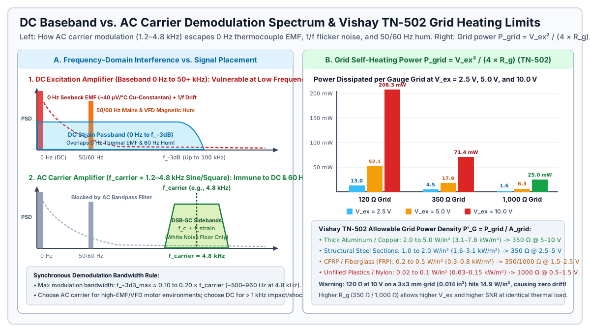
Engineering Parameter	DC Excitation Bridge Conditioner	AC Carrier Synchronous Demodulator (1.2–4.8 kHz)	Practical Selection Consequence
Maximum Usable Signal Bandwidth (f_-3dB)	0 Hz (DC) up to 50 kHz – 250 kHz (22.5 kHz on NI-9237; 100+ kHz on wideband analog INAs)	Bounded to 0.10 to 0.20 × f_carrier (~120 Hz on a 600 Hz carrier; ~500 Hz to 960 Hz on a 4.8 kHz carrier)	Mandatory to use DC excitation for signals above 1 kHz (shock, crash, ballistics, blade passing)
Thermoelectric (Seebeck) Parasitic EMF Rejection	Vulnerable: Copper wire soldered to Constantan tabs forms a ~40 μV/°C thermocouple at 0 Hz (16 με/°C error on a 5 V quarter bridge)	Immune: 0 Hz thermocouple voltages are blocked by the AC input stage and rejected by synchronous demodulation	Use AC carrier (or reversing DC pulse excitation) when thermal gradients exist across solder tabs or connectors
50 Hz / 60 Hz Mains & VFD Motor Magnetic Hum	Normal-mode magnetic loop pickup inside the passband passes directly into the ADC output	> 100 to 120 dB rejection: 50/60 Hz hum lies far outside the 4.8 kHz carrier bandpass window	Use AC carrier near 480 V VFD motor drives, welding lines, induction heaters, or electric traction rigs
Amplifier 1/f Flicker Noise & Zero Drift	Baseband amplification intersects 1/f semiconductor flicker noise unless chopper-stabilized	Amplifies at 4.8 kHz in the flat white-noise region above the 1/f corner, yielding sub-nanovolt zero stability	AC carrier excels in multi-month geotechnical, bridge weigh-in-motion, and creep tests
Cable Capacitance & Phase Balance Sensitivity	Insensitive to steady-state cable shunt capacitance (only limits upper -3 dB corner)	Sensitive to capacitive asymmetry (C_cable), requiring resistive (R) and reactive quadrature (C) phase auto-balance	Long cables on AC carrier systems require shielded twisted-pair cabling with stable capacitance

Takeaway: Choose DC excitation whenever your mechanical bandwidth exceeds 500 Hz (see our DAQ vs oscilloscope transient capture guide); choose an AC carrier conditioner when 0 Hz thermocouple drift or 50/60 Hz magnetic interference corrupts low-frequency microstrain stability.

How Do 6-Wire Kelvin Sense, Shunt Calibration, and Anti-Aliasing Filters Prevent Span and Peak Errors?

Even with an ideal instrumentation amplifier, three external signal-chain mechanisms can invalidate your strain or force data before the bits reach disk: leadwire series resistance (R_lead), unverified amplifier gain scaling, and anti-aliasing filter overshoot or Nyquist folding.

Leadwire Desensitization and 6-Wire Kelvin Remote Sensing

Copper instrumentation cable has a nominal resistance of 84.2 Ω/km (2.57 Ω/100 ft) for 24 AWG (0.20 mm^2) or 133.9 Ω/km (4.08 Ω/100 ft) for 26 AWG (0.14 mm^2), combined with a high temperature coefficient of resistance α_Cu = +0.00393 /°C (+0.393%/°C, or ~22% per 55°C / 100°F). Whenever copper lead resistance sits in series with the bridge excitation or active gauge arm, it divides down the excitation voltage reaching the strain-sensitive foil grid.

For single-grid surface installations, our three-wire quarter-bridge checks guide shows how moving from a 2-wire to a 3-wire hookup splits the two current-carrying leads into adjacent arms (R_g + R_L1 and R_4 + R_L2), canceling leadwire thermal zero drift and cutting span loss from 2 × R_lead / (R_g + 2 × R_lead) down to R_lead / (R_g + R_lead). For full-bridge transducers and load cells, moving from a 4-wire cable to a 6-wire Kelvin remote sense cable eliminates leadwire span error completely.

Bridge Wiring Topology	Span Attenuation Factor (K_lead = V_measured / V_ideal)	Fractional Span Error (e_lead)	Leadwire Thermal Zero Drift	Leadwire Thermal Span Drift (α_Cu = +0.393%/°C)
2-Wire Quarter-Bridge	R_g / (R_g + 2 × R_lead)	-(2 × R_lead) / (R_g + 2 × R_lead)	Severe (156 με per 5.5°C on 6 m of 26 AWG with 120 Ω gauge per Vishay TT-612)	Uncompensated
3-Wire Quarter-Bridge (R_L1 = R_L2)	R_g / (R_g + R_lead)	-R_lead / (R_g + R_lead)	Canceled when R_L1 and R_L2 share length, AWG, and cable jacket temperature	Half of 2-wire span drift (R_lead remains in series with R_g)
4-Wire Full-Bridge (R_bridge = R_g)	R_bridge / (R_bridge + 2 × R_lead)	-(2 × R_lead) / (R_bridge + 2 × R_lead)	Canceled by full-bridge symmetry	Uncompensated (-1.41% span loss on 30 m 24 AWG with 350 Ω bridge)
6-Wire Full-Bridge with Kelvin Sense (+Exc, -Exc, +Sense, -Sense, +Sig, -Sig)	1.0000 (within excitation regulator compliance or ratiometric ADC range)	0.00%	Canceled by full-bridge symmetry	Canceled (0.00%/°C via active remote sense or ratiometric V_ref)

Worked Example 2: 4-Wire vs. 6-Wire Kelvin Sense on a 30 m (100 ft) Load Cell Cable

Consider a 350 Ω full-bridge strain gauge force sensor (2.000 mV/V rated output) connected to a strain gauge amplifier at the end of a 30 m (100 ft) 24 AWG copper cable (R_lead = 2.50 Ω per conductor, or 2 × R_lead = 5.00 Ω round-trip excitation loop) with a 5.000 V excitation setting:

Case A: 4-Wire Full-Bridge Connection (No Sense Lines)
• Total loop resistance seen by excitation source: R_total = 350.0 Ω + 2 × 2.50 Ω = 355.0 Ω
• Excitation current: I_bridge = 5.000 V / 355.0 Ω = 14.085 mA
• Voltage drop lost across excitation leads: V_drop = 14.085 mA × 5.00 Ω = 70.42 mV
• Actual voltage reaching bridge terminals: V_ex_bridge = 5.000 V - 0.07042 V = 4.9296 V
• Full-scale bridge signal: V_out = 4.9296 V × 2.000 mV/V = 9.859 mV (instead of 10.000 mV)
• Systematic span error: e_lead = -5.00 / (350.0 + 5.00) = -1.408% (-140.8 N error on a 10 kN load cell!)
• Plus thermal span shift if cable warms by ΔT = +20°C:
  ΔR_loop = 5.00 Ω × 0.00393 /°C × 20°C = +0.393 Ω => additional -0.11% span drift.

Case B: 6-Wire Kelvin Remote-Sensed Connection (+Sense and -Sense Landed at Transducer)
• High-impedance Kelvin sense inputs draw negligible current (< 1 nA), so I_sense × R_lead ≈ 0 V.
• Active Regulator Mode: Conditioner senses V(+Sense) - V(-Sense) and boosts source output to
  5.0714 V so that V_ex_bridge at the load cell terminals is held at exactly 5.000 V.
• Ratiometric ADC Mode (e.g., NI-9237 / PXIe-4330): ADC measures V_out / [V(+Sense) - V(-Sense)]
  = 9.859 mV / 4.9296 V = 2.0000 mV/V exact.
• Systematic span error: 0.000%, independent of cable length and ambient cable temperature.

If a long industrial cable run must feed a PLC analog input that lacks 6-wire Kelvin sense, place a local DIN-rail bridge conditioner next to the load cell and convert the signal to a current loop as detailed in our 4-20 mA sensor DAQ wiring guide.

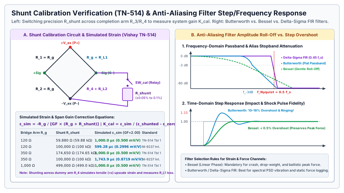
Worked Example 3: Shunt Calibration Verification and Gain Correction (K_cal)

Per Vishay Micro-Measurements Tech Note TN-514 (Shunt Calibration of Strain Gage Instrumentation), shunt calibration verifies the entire signal conditioning channel (including R_lead attenuation and amplifier gain G) by switching a precision resistor R_shunt (±0.05% to ±0.1% tolerance, <= 25 ppm/°C) in parallel with one arm of the bridge (R_g). Shunting R_g with R_shunt lowers that arm’s resistance to R_p = (R_g × R_shunt) / (R_g + R_shunt), producing an exact fractional resistance change ΔR / R_g = -R_g / (R_g + R_shunt) and a simulated mechanical strain ε_sim:

ε_sim (in m/m) = -R_g / [GF × (R_g + R_shunt)]
με_sim         = -10^6 × R_g / [GF × (R_g + R_shunt)]

Required R_shunt for target |ε_sim|:
R_shunt = [R_g / (GF × |ε_sim|)] - R_g

Suppose you activate the internal 100.0 kΩ (100,000 Ω) solid-state shunt calibration switch on an NI-9237 or PXIe-4330 module connected to a 350.0 Ω bridge arm with package gauge factor GF = 2.000 over a 3-wire cable with R_lead = 2.50 Ω per conductor:

1. Calculate ideal simulated microstrain (with R_g = 350.0 Ω, R_shunt = 100,000 Ω, GF = 2.000):
   με_sim = -10^6 × 350.0 / [2.000 × (350.0 + 100,000)]
          = -350,000,000 / 200,700
          = -1,743.90 με (equivalent to 0.87195 mV/V upscale when shunted across completion arm R_4)

   (Note: Using the Vishay TN-514 Table 1 standard resistor R_shunt = 174,650 Ω on 350 Ω gives:
    με_sim = -10^6 × 350.0 / [2.000 × (350.0 + 174,650)] = -1,000.00 με exact.)

2. Record unstrained zero reading (SW_cal OPEN):
   ε_zero = +1.20 με

3. Close shunt switch across completion arm R_4 (SW_cal CLOSED) and read uncalibrated channel output:
   Because R_lead = 2.50 Ω sits in series with the active gauge, the uncalibrated channel reads:
   ε_shunted = +1,732.73 με
   Δε_measured = ε_shunted - ε_zero = 1,732.73 - 1.20 = 1,731.53 με

4. Compute and apply the channel Gain Correction Factor K_cal:
   K_cal = |με_sim| / Δε_measured = 1,743.90 / 1,731.53 = 1.00714 (+0.714% span correction)

Selecting Anti-Aliasing Low-Pass Filters: Butterworth vs. Bessel vs. Delta-Sigma FIR

Every strain gauge amplifier must band-limit its analog output before sampling at rate f_s so that high-frequency mechanical resonances, structural ringing, and electromagnetic noise above the Nyquist folding frequency (f_Nyquist = f_s / 2) do not alias back into the measurement passband. For multi-channel sample-rate and storage calculations, see our DAQ sample rate planning worksheet.

Filter Topology	Amplitude Passband & Roll-Off	Phase Linearity & Group Delay	Step-Response Overshoot	Recommended Strain / Force Application
4- to 8-Pole Butterworth Low-Pass	Maximally flat passband amplitude (< 0.01 dB ripple to 0.7 × f_-3dB); sharp -80 to -160 dB/decade roll-off	Nonlinear phase near f_-3dB	10% to 18% overshoot with damped ringing	Frequency-domain vibration PSD analysis, sine-sweep fatigue, and quasi-static weighing (set f_s >= 5 to 10 × f_-3dB)
4- to 8-Pole Bessel Low-Pass	Gradual amplitude droop starting below 0.5 × f_-3dB; slower stopband roll-off	Maximally flat group delay (linear phase across passband)	< 0.5% overshoot (zero ringing)	Time-domain crash sleds, drop-weight impact tups, Charpy testing, and peak force capture (set f_s >= 10 × f_-3dB)
24-Bit Delta-Sigma Digital FIR (NI-9237, PXIe-4330)	Brick-wall flat passband to 0.45 × f_s (±0.1 dB); > 100 dB alias rejection at 0.55 × f_s	Strictly linear phase; deterministic constant group delay (~38 to 40 samples)	Symmetric Gibbs pre- and post-ringing on steps faster than 0.45 × f_s	Simultaneous multi-channel bridge DAQ; compensate for the 39 / f_s group delay (0.78 ms at 50 kS/s) in real-time control loops

Takeaway: Never place a steep analog Butterworth filter on a crash or impact force sensor channel without accounting for its 10% to 18% step-response overshoot; select a linear-phase Bessel filter and oversample at f_s >= 10 × f_-3dB whenever time-domain peak force accuracy governs the test.

Pre-Acquisition Commissioning Checklist for Bridge Amplifier Channels

Before logging mechanical test data, execute this six-point verification sequence on each conditioned channel:

1. Verify gauge resistance and thermal power density: Measure unbonded or unmounted bridge resistance (120 Ω, 350 Ω, or 1,000 Ω) with a four-wire ohmmeter, compute P'_G = V_ex^2 / (4 × R_g × A_grid), and confirm V_ex stays within the Vishay TN-502 limit for your specimen substrate (<= 2.5 V for 120 Ω on steel; <= 1.5 V on composites).
2. Confirm 3-wire or 6-wire Kelvin remote sense continuity: Verify that +Sense and -Sense connect directly at the load cell or remote bridge excitation corners rather than being jumpered at the DAQ front panel when cable length exceeds 3 m (10 ft).
3. Measure unstrained bridge zero offset before software tare: Record raw differential mV/V offset with the structure unloaded. An offset exceeding ±1.0 mV/V on a foil installation or ±2% of rated output on a strain gauge force sensor indicates yielding, installation pre-strain, or leadwire asymmetry rather than an amplifier calibration shift.
4. Match amplifier gain G to maximum expected peak load (including dynamic impact margin): Size G = V_ADC_FS / (V_ex × V_r_peak) with 20% to 30% headroom below the instrumentation amplifier output rail and ADC saturation voltage.
5. Execute a two-point shunt calibration check (SW_cal open vs. closed): Compare the measured shunt step Δε_measured against ε_sim = -R_g / [GF × (R_g + R_shunt)], verify that K_cal matches expected leadwire attenuation 1 + (R_lead / R_g), and confirm the reading returns to 0.0 ± 0.5 με when the shunt switch opens.
6. Record anti-aliasing filter type, -3 dB cutoff, and group delay: Log whether the channel uses a Bessel, Butterworth, or Delta-Sigma FIR filter alongside sampling rate f_s so time-aligned channels share identical phase delay.

Threshold rule: Whenever cable length exceeds 3 m (10 ft) on a 120 Ω or 350 Ω bridge, or whenever ambient cable temperature varies by more than ±5°C, wire 6-wire Kelvin remote sense on full bridges and 3-wire completion with shunt calibration across the completion arm on quarter bridges.

Takeaway: Complete the excitation power check, remote sense verification, unloaded zero measurement, and two-point shunt step before every test series so cable resistance and amplifier gain errors are corrected in hardware rather than estimated after the test.