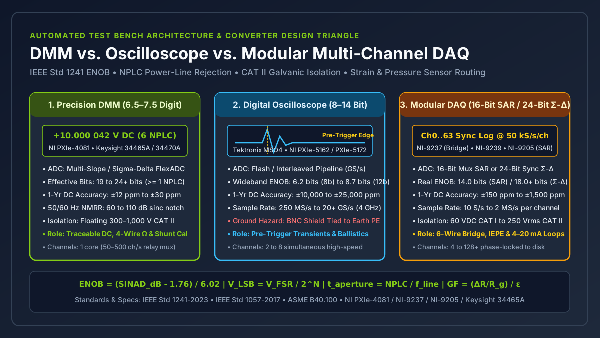
An automated test bench partitions measurements across three distinct converter architectures: a precision digital multimeter (DMM) for power-line-rejected floating DC and four-wire resistance standards, a digital storage oscilloscope (DSO) for gigasample-per-second pre-trigger transient capture, and a modular multi-channel data acquisition (DAQ) system for synchronized sensor conditioning and continuous disk logging. Treating a DMM, an oscilloscope, and a modular DAQ as interchangeable voltage readers causes severe quantization error on microvolt bridge signals, unattenuated 50/60 Hz mains ripple when sampling below one power-line cycle, or a 5 A to 20 A ground-loop fault current when an earth-bonded oscilloscope BNC shield is clipped to a floating shunt or bridge leg.
Assign each test bench channel by evaluating four hardware boundaries in order: calculate required Effective Number of Bits (ENOB = (SINAD_dB - 1.76) / 6.02) against minimum signal step V_LSB = V_FSR / 2^ENOB, select an integer power-line integration aperture (t_aperture = NPLC / f_line, 100 ms universal window) whenever normal-mode 50/60 Hz rejection (>= 60 to 110 dB NMRR) governs DC stability, verify galvanic isolation between earth-referenced BNC shields and floating CAT II 300 V to 1,000 V terminals, and match the transducer physics (how does strain gauge work and pressure gauge types) to ratiometric bridge, 4–20 mA shunt, or AC-coupled IEPE conditioning.
This architecture guide belongs to the Sensors and DAQ engineering hub, extends our DAQ vs oscilloscope requirements boundary guide into converter physics and multi-instrument PXIe/CompactDAQ racks, and pairs with our strain gauge amplifier signal conditioning and bandwidth guide. Maximizing Value at NI is an independent technical resource (about this site) not affiliated with National Instruments (NI) or Emerson.
| Architectural Metric | 6.5–7.5 Digit Precision DMM (NI PXIe-4081, Keysight 34465A) |
8–12 Bit Digital Storage Oscilloscope (Tektronix MSO4, NI PXIe-5162) |
16-Bit Multiplexed SAR DAQ (NI-9205, PXIe-6363) |
24-Bit Simultaneous Delta-Sigma DAQ (NI-9237, NI-9239) |
|---|---|---|---|---|
| Primary ADC Topology | Multi-slope integrating or Sigma-Delta FlexADC with line-locked decimation | Parallel Flash, interleaved pipeline, or high-speed SAR ADC | CMOS analog multiplexer + PGIA + single shared 16-bit SAR ADC | 1 dedicated oversampled 24-bit Delta-Sigma modulator + digital FIR per channel |
Nominal Resolution (N) |
6.5 to 7.5 digits (2,000,000 to 20,000,000 counts, 21 to 26 bits) |
8 bits (256 levels), 10 bits (1,024), or 12 bits (4,096 levels) |
16 bits (65,536 vertical levels) |
24 bits (16,777,216 vertical levels) |
Real-World Wideband ENOB (IEEE 1241) |
19.0 to 23.5+ bits (at >= 1 NPLC DC aperture) |
6.2 bits (8-bit DSO) to 8.7 bits (12-bit HD DSO across full BW) |
13.8 to 14.2 bits (settling-limited when mux scanning) |
17.8 to 19.5 bits (109 to 119 dB dynamic range) |
Effective Step on ±10 V Range (V_FSR = 20 V) |
< 1.0 μV (100 nV on 1 V range at 100 ms aperture) |
272.0 mV (6.2 ENOB) to 48.1 mV (8.7 ENOB) |
1.22 mV (305.2 μV nominal LSB; 6.10 μV on ±200 mV PGIA range) |
76.3 μV (18.0 ENOB on ±10 V); 29.8 nV nominal LSB on NI-9237 (±25 mV/V) |
Sampling Rate (f_s) |
0.01 S/s (100 NPLC) to 50 kS/s (1.8 MS/s in PXIe-4081 digitizer mode) |
250 MS/s to 20+ GS/s (50 ps to 4 ns sample interval) |
250 kS/s to 2 MS/s aggregate (f_s / N_ch per scanned channel) |
10 S/s to 51.2 kS/s per channel simultaneous (0.45 × f_s alias-free BW) |
| 1-Year DC Voltage Accuracy | ±12 ppm to ±30 ppm (0.0012% to 0.0030%) |
±10,000 ppm to ±25,000 ppm (1.0% to 2.5% of full scale) |
±150 ppm to ±620 ppm (±6.23 mV at ±10 V full scale on NI-9205) |
±150 ppm to ±500 ppm (±0.05% ratiometric gain error on NI-9237) |
50 Hz / 60 Hz Normal-Mode Rejection (NMRR) |
>= 60 dB at 1 NPLC; 80 to 110 dB at >= 5 NPLC (100 ms window) |
0 dB (passes 50/60 Hz power-line hum directly into waveform) |
0 dB in passband (requires software post-filter or shielding) |
0 dB in passband (> 100 dB out-of-band alias rejection at 0.55 × f_s) |
| Input Grounding & Isolation Rating | Floating HI/LO (300 V to 1,000 V CAT I / CAT II channel-to-earth) |
Earth-bonded BNC shield (0 V isolation without active differential probe) |
Differential + 60 VDC CAT I (D-SUB) or 250 Vrms CAT II (spring terminal) |
Differential + 60 VDC CAT I bank (NI-9237) to 250 Vrms CAT II ch-to-ch (NI-9239) |
| Primary Test Bench Role | Traceable DC reference, 4-wire Kelvin ohms, and precision shunt current | High-speed edge/glitch triggers, eye diagrams, and MHz ballistic shock | High-channel-count 0–10 V and 4–20 mA industrial process scanning |
Ratiometric mV/V strain bridges, load cells, and IEPE vibration arrays |
Takeaway: Partition your measurement rack along converter physics rather than software convenience: route microvolt DC accuracy and 4-wire ohms to the DMM, nanosecond pre-trigger transients to the oscilloscope, and phase-synchronized multi-sensor arrays to the modular DAQ.
Why Does DMM vs Oscilloscope vs DAQ Architecture Split Across Sample Rate and ENOB?
Evaluating dmm vs oscilloscope and modular DAQ specifications requires looking past datasheet nominal bit counts (8-bit, 16-bit, 24-bit) to the physical trade-off between sampling speed (f_s) and Effective Number of Bits (ENOB). Every analog-to-digital converter is bounded by thermal resistor noise (e_n = sqrt(4 × k_B × T × R × B)), comparator ambiguity, harmonic distortion in the analog front-end preamplifier, and sample-clock aperture jitter (t_j).
Per IEEE Std 1241-2023 (IEEE Standard for Terminology and Test Methods for Analog-to-Digital Converters) and IEEE Std 1057-2017 (IEEE Standard for Digitizing Waveform Recorders), an ideal N-bit converter dividing a full-scale peak-to-peak input span V_FSR produces 2^N discrete quantization levels separated by one Least Significant Bit (V_LSB):
Nominal Quantization Step:
V_LSB = V_FSR / 2^N

Ideal RMS Quantization Noise (uniformly distributed across [-0.5 LSB, +0.5 LSB]):
e_q_rms = V_LSB / sqrt(12)

Theoretical Maximum SNR of an Ideal N-Bit Converter (for full-scale sine wave):
SNR_ideal_dB = 6.0206 × N + 1.7609 dB

IEEE Std 1241 Signal-to-Noise-and-Distortion Ratio (SINAD) and Effective Number of Bits (ENOB):
SINAD_dB = 20 × log10( V_signal_rms / sqrt(V_noise_rms^2 + V_THD_rms^2) )
ENOB     = (SINAD_dB - 1.76) / 6.02

Effective Noise-Free Voltage Resolution Step:
V_res_eff = V_FSR / 2^ENOB
When an oscilloscope front end opens its -3 dB analog bandwidth to 500 MHz or 1.5 GHz (NI PXIe-5162, Tektronix MSO4) to capture sub-nanosecond edges, integrated wideband thermal noise (sqrt(B)) and gigahertz clock jitter raise V_noise_rms and drop real-world ENOB by 1.8 to 3.3 bits below the nominal ADC rating. Conversely, when a 24-bit Delta-Sigma DAQ (NI-9237, NI-9239) or a 7.5-digit DMM (NI PXIe-4081, Keysight 34465A) oversamples the input with a modulator and applies a steep digital decimation filter or multi-cycle line integration window, out-of-band noise is stripped away, pushing ENOB to 18 to 24 bits.
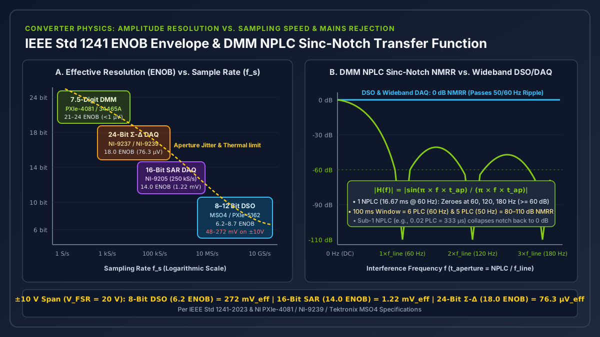
Worked Example 1: Resolving a Millivolt Sensor Shift on a ±10 V Span (V_FSR = 20.0 V)
Suppose an automated test sequence monitors a ±10.0 V bipolar range (V_FSR = 20.0 V peak-to-peak) while attempting to resolve a 100.0 μV (0.10 mV) DC shift from a pressure or force sensor conditioner:
1. 8-Bit Digital Storage Oscilloscope (Nominal N = 8, 256 levels; SINAD = 39.1 dB at 500 MHz):
   • Nominal step:   V_LSB     = 20.0 V / 2^8   = 20.0 V / 256        = 78.125 mV
   • Real-world ENOB: ENOB     = (39.1 - 1.76) / 6.02                 = 6.20 bits (73.5 levels)
   • Effective step: V_res_eff = 20.0 V / 2^6.20                      = 272.0 mV
   • Consequence: A 100 μV shift is 2,720× smaller than the scope's effective step on ±10 V.
     Even at max vertical zoom (1 mV/div × 8 div = 8.0 mV full scale), V_LSB = 31.25 μV and
     wideband front-end noise (~150 to 300 μVrms) completely buries a 100 μV static shift.

2. 12-Bit High-Definition Oscilloscope (Nominal N = 12, 4,096 levels; SINAD = 54.1 dB):
   • Nominal step:   V_LSB     = 20.0 V / 2^12  = 20.0 V / 4,096      = 4.883 mV
   • Real-world ENOB: ENOB     = (54.1 - 1.76) / 6.02                 = 8.70 bits (416 levels)
   • Effective step: V_res_eff = 20.0 V / 2^8.70                      = 48.1 mV
   • Consequence: 16× finer quantization than an 8-bit scope for viewing switching ripple or
     hydraulic transient peaks, yet still 481× too coarse for a 100 μV static step on ±10 V.

3. 16-Bit Multiplexed SAR DAQ (NI-9205, Nominal N = 16, 65,536 levels; ENOB = 14.0 bits):
   • Nominal step on ±10 V:    V_LSB     = 20.0 V / 65,536            = 305.18 μV
   • Effective step on ±10 V:  V_res_eff = 20.0 V / 2^14.0            = 1.221 mV
   • Switching internal PGIA to ±200 mV range (V_FSR = 0.400 V):
     V_LSB = 0.400 V / 65,536 = 6.104 μV (RMS noise ~8.0 μVrms), resolving 100 μV with a 12.5:1 SNR.

4. 24-Bit Simultaneous Delta-Sigma DAQ (NI-9239, Nominal N = 24, 16,777,216 levels; SINAD = 110.1 dB):
   • Nominal step on ±10 V:    V_LSB     = 20.0 V / 16,777,216        = 1.192 μV
   • Real-world ENOB:          ENOB      = (110.1 - 1.76) / 6.02      = 18.00 bits (262,144 levels)
   • Effective step on ±10 V:  V_res_eff = 20.0 V / 2^18.00           = 76.29 μV across full ±10 V!
   • On NI-9237 (±25 mV/V bridge range at V_ex = 10 V => V_FSR = 0.500 V):
     Nominal V_LSB = 0.500 V / 2^24 = 29.80 nV, resolving sub-microvolt bridge changes directly.

5. 7.5-Digit Precision DMM (NI PXIe-4081 / Keysight 34470A at 100 ms / 6 NPLC aperture):
   • On ±10 V range: 20,000,000 counts (24.25 bits), least count = 1.0 μV (0.1 μV on 1 V range),
     with ±15 ppm 1-year absolute DC accuracy (±150 μV total uncertainty at 10.000000 V).
Takeaway: Never rely on nominal bit depth alone; compute V_res_eff = V_FSR / 2^ENOB on the active input range to verify that your smallest required physical measurement step exceeds the converter’s effective noise floor by at least a factor of 4 to 10.
How Does DMM NPLC Aperture Integration Reject 50/60 Hz Mains Hum That Corrupts Oscilloscopes?
In industrial test cells, unshielded power transformers, variable-frequency motor drives, and fluorescent lighting couple 50 Hz or 60 Hz sinusoidal interference (V_noise × sin(2π × f_line × t + φ)) onto sensor leads. An oscilloscope or wideband SAR DAQ samples the input with a sub-microsecond sample-and-hold aperture (t_SH < 100 ns), which is designed to capture AC waveforms faithfully. Consequently, an oscilloscope or wideband DAQ has 0 dB intrinsic Normal-Mode Rejection Ratio (NMRR) at 50 Hz / 60 Hz: every millivolt of power-line ripple rides directly into the digitized record.
A precision integrating DMM eliminates power-line hum in hardware by integrating the input voltage over a rectangular time window t_aperture scaled in NPLC (Number of Power Line Cycles):
Integration Aperture Duration:
t_aperture = NPLC / f_line

Normalized Sinc Frequency Response of Rectangular Integration Window:
|H(f)| = | sin(π × f × t_aperture) / (π × f × t_aperture) |

Normal-Mode Rejection Ratio (in dB) at Interference Frequency f:
NMRR_dB(f) = -20 × log10( | sin(π × f × t_aperture) / (π × f × t_aperture) | )
Whenever NPLC is set to an integer M = 1, 2, 5, 6, 10, 100 (t_aperture = M / f_line) and the interference frequency f is an integer harmonic k × f_line (60 Hz, 120 Hz, 180 Hz... or 50 Hz, 100 Hz, 150 Hz...), the argument inside the sine function becomes π × (k × f_line) × (M / f_line) = π × k × M. Because sin(π × integer) = 0, the positive half-cycle and negative half-cycle of the AC mains sine wave sum to zero over the integration window, placing an exact mathematical transmission zero (|H(k × f_line)| = 0) across the fundamental power-line frequency and all of its harmonics.
DMM Integration Setting (NPLC) |
Aperture Time t_aperture (@ 60 Hz / @ 50 Hz) |
Effective -3 dB Bandwidth (0.443 / t_aperture) |
Theoretical NMRR at ±0.1% Grid Frequency Drift |
Max Reading Rate (Single Channel, Auto-Zero Off/On) | Recommended Test Bench Task |
|---|---|---|---|---|---|
0.006 NPLC (Fast Digitizing) |
100 μs (60 Hz) / 120 μs (50 Hz) |
4,430 Hz (60 Hz) |
0.00 dB (no line cycle integration) |
10,000 to 50,000 S/s |
High-speed pulsed power & relay bounce capture |
0.1 NPLC (High-Speed Scan) |
1.667 ms (60 Hz) / 2.000 ms (50 Hz) |
265.8 Hz (60 Hz) |
0.14 dB (passes 50/60 Hz hum) |
500 to 600 S/s |
Low-impedance DC rail checks in shielded enclosures |
1.0 NPLC (Standard Production) |
16.667 ms (60 Hz) / 20.000 ms (50 Hz) |
26.58 Hz (60 Hz) / 22.15 Hz (50 Hz) |
>= 60.0 dB (1,000:1 ripple attenuation) |
60 S/s (30 S/s with Auto-Zero) |
Automated production ATE resistance & DC voltage |
5 NPLC (50 Hz) / 6 NPLC (60 Hz) |
100.000 ms (Universal 50/60 Hz Window) |
4.43 Hz |
>= 80 to 110 dB (with high-order digital window) |
10 S/s (5 S/s with Auto-Zero) |
Universal global test racks (NI PXIe-4081 default precision window) |
100 NPLC (Metrology Reference) |
1.667 s (60 Hz) / 2.000 s (50 Hz) |
0.266 Hz (60 Hz) |
>= 100 to 120 dB |
0.6 S/s (0.3 S/s with Auto-Zero) |
Sub-ppm calibration transfer standards & nanovolt checks |
Worked Example 2: 1 NPLC vs. 0.02 NPLC Mains Hum Rejection Under ±0.1% Grid Drift
Suppose a 10.0000 V DC sensor signal carries 100.0 mV peak (200 mVpp) of 60 Hz magnetic induction hum, and the local utility grid drifts by +0.10% to f = 60.060 Hz:
Case A: DMM set to 0.02 NPLC for fast scanning (t_aperture = 0.02 / 60 Hz = 333.33 μs)
• Sinc argument: x = π × 60.060 Hz × 0.00033333 s = 0.06289 radians
• Attenuation:   |H(60.06 Hz)| = |sin(0.06289) / 0.06289| = 0.99934 (NMRR = 0.006 dB)
• Residual error: 100.0 mV × 0.99934 = ±99.93 mV peak ripple directly corrupts the reading!

Case B: DMM set to 1.0 NPLC (t_aperture = 1.0 / 60 Hz = 16.6667 ms)
• Sinc argument: x = π × 60.060 Hz × 0.0166667 s = 1.00100 × π radians
• Attenuation:   |H(60.06 Hz)| = |sin(1.001 × π) / (1.001 × π)| = 0.0031416 / 3.14473 = 0.000999
• NMRR:          -20 × log10(0.000999) = 60.01 dB (1,001:1 attenuation)
• Residual error: 100.0 mV × 0.000999 = ±99.9 μV peak error (a 1,000× reduction in mains noise).

Case C: NI PXIe-4081 set to 100.0 ms Universal Aperture with High-Order DC Noise Rejection
• 100.0 ms equals exactly 6.00 PLC at 60 Hz (6 × 16.6667 ms) AND 5.00 PLC at 50 Hz (5 × 20.000 ms).
• Achieves >= 100 dB NMRR (< 1.0 μV residual error from 100 mV peak hum) on both 50 Hz and 60 Hz
  power grids simultaneously without changing test software parameters.
Takeaway: Always configure precision DC voltage and 4-wire resistance checks to >= 1 NPLC (or 100 ms universal aperture for global racks); dropping below 1 NPLC collapses the sinc notch to 0 dB and admits full peak-to-peak mains hum.
How Do Ground Loops and BNC Shield Short Circuits Differ Across Oscilloscopes, DMMs, and DAQs?
Before connecting any probe or terminal block, verify the input reference and galvanic isolation topology of the instrument. As established in our floating DAQ input wiring and common-mode guide, landing a single-ended earth-grounded input on a non-zero common-mode node causes either measurement corruption or catastrophic hardware damage.
On virtually every standard benchtop oscilloscope (Tektronix MSO4, Keysight InfiniiVision) and modular PXIe oscilloscope (NI PXIe-5162, PXIe-5172), the outer metal shell of every front-panel BNC connector is bonded directly to the instrument chassis and, through the three-prong IEC power cord, to building Protective Earth (PE, R_PE < 0.1 Ω). All passive oscilloscope probe alligator ground clips are tied together and tied to earth ground.
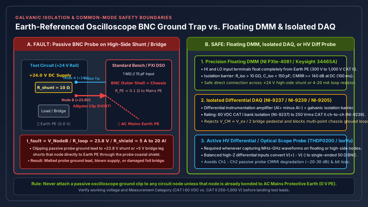
Worked Example 3: The High-Side Shunt and Bridge BNC Ground-Clip Short Circuit
Suppose an engineer needs to measure the current drawn by an industrial actuator on a +24.0 V DC supply rail across a high-side sense resistor R_shunt = 10.0 Ω carrying I_load = 20.0 mA (V_shunt = 200.0 mV, so Node A = +24.0 V and Node B = +23.8 V relative to earth ground), or across the differential signal corners (+Sig and -Sig sitting at a +5.0 V common-mode pedestal) of an earth-referenced Wheatstone bridge:
Fault Scenario: Connecting a Standard Passive Oscilloscope Probe Across R_shunt
• Probe tip landed on Node A (+24.0 V); probe alligator ground clip landed on Node B (+23.8 V).
• Because the alligator clip is bonded to Protective Earth (0.0 V PE) via coaxial shield resistance
  R_shield ≈ 0.35 Ω and power cord ground R_PE ≈ 0.08 Ω (R_loop ≈ 0.43 Ω):
  Node B (+23.8 V) is shorted directly to Earth Ground!
• Fault current through probe ground lead:
  I_fault = 23.8 V / 0.43 Ω = 55.3 A (clamped only by the 24 V power supply current limit, typically 5 A to 20 A).
• Consequence: The 5 A to 20 A fault current melts the passive probe ground lead and coaxial shield,
  trips or destroys the 24 V supply, or vaporizes the 350 Ω foil grid when clipped to a bridge leg.

Safe Architecture 1 (DC to Low-kHz): Floating DMM (NI PXIe-4081 / Keysight 34465A)
• Both HI and LO terminals are galvanically isolated from Earth PE up to 300 V / 1,000 V CAT II
  (DC isolation resistance R_iso > 10 GΩ, isolation capacitance C_iso < 150 pF, CMRR >= 140 dB).
• Landing LO on Node B (+23.8 V) draws < 2.4 nA DC leakage and reads V_shunt = +200.000 mV safely.

Safe Architecture 2 (Multi-Channel DC to 50 kHz): Isolated Differential DAQ (NI-9239 / NI-9237 / NI-9205)
• High-impedance differential instrumentation amplifier measures V(AI+) - V(AI-) across an optical or
  capacitive isolation barrier rated at 60 VDC CAT I (NI-9237) or 250 Vrms CAT II channel-to-channel (NI-9239).

Safe Architecture 3 (MHz to GHz Transients): Active High-Voltage Differential Probe on Oscilloscope
• Leave passive ground clips disconnected from floating nodes; use an active differential probe
  (e.g., Tektronix THDP0200 / TDP1000 or Keysight N2790A) with balanced high-impedance inputs
  that reject the +23.8 V common-mode rail and drive the scope's earth-referenced 50 Ω BNC safely.
Takeaway: Never clip a passive oscilloscope ground lead to any circuit point that is not already bonded to 0.0 V Protective Earth; use a floating DMM or isolated differential DAQ below 50 kHz, and an active differential probe for megahertz transients.
How Does a Strain Gauge Work and Which Instrument Captures Bridge Signals Accurately?
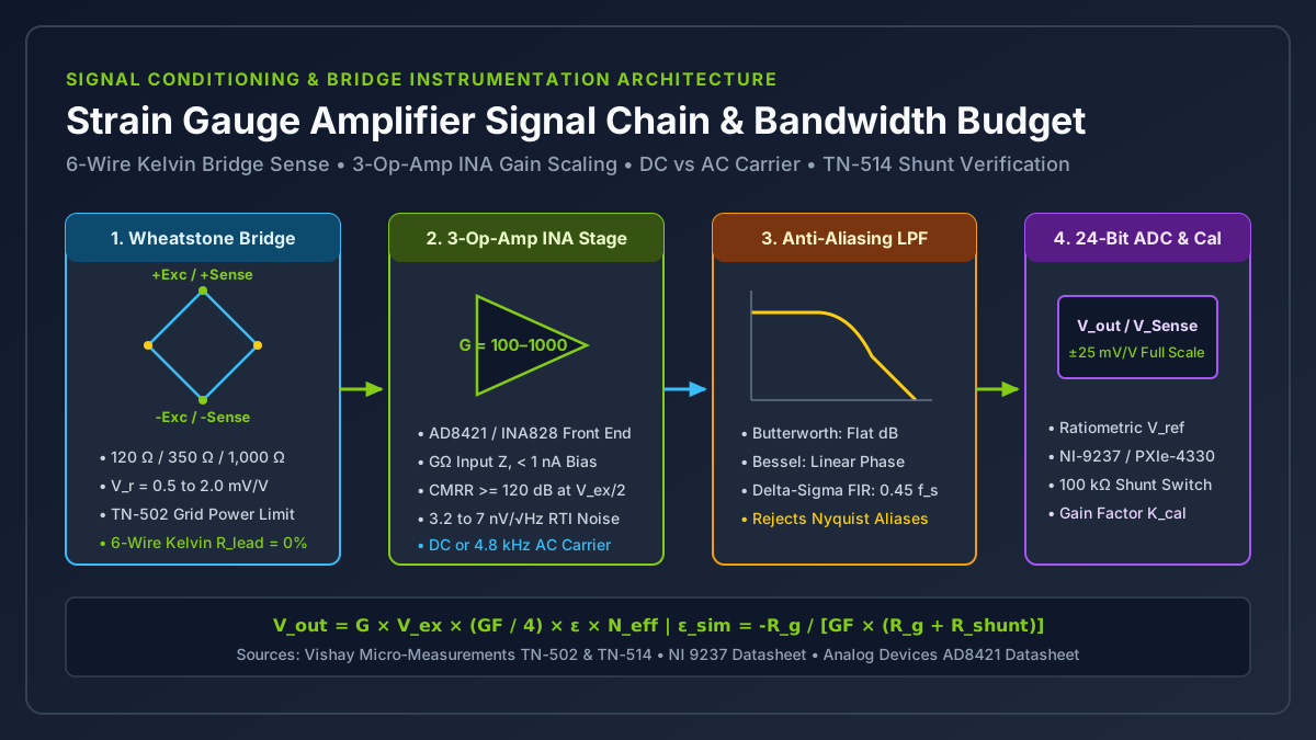
Understanding how does strain gauge work explains why raw structural sensors cannot simply be plugged into a general-purpose oscilloscope or unconditioned voltage DAQ. As derived in our strain gauge basics and gauge factor guide and Wheatstone bridge quarter, half, and full bridge guide, a metallic foil strain gauge consists of a photo-etched Constantan (55% Cu / 45% Ni) or Modified Karma (Ni-Cr) resistive grid (R_g = 120 Ω, 350 Ω, or 1,000 Ω) bonded to an insulating polyimide backing.
When the structural specimen deforms under mechanical strain ε = ΔL / L (expressed in microstrain με = ε × 10^6, where 1,000 με = 0.10% length change), the bonded foil grid elongates or contracts, changing its electrical resistance ΔR according to the Gauge Factor (GF):
Fundamental Piezoresistive Strain Gauge Equation:
GF = (ΔR / R_g) / ε     =>     ΔR = R_g × GF × ε

Wheatstone Bridge Ratiometric Output Voltage (excited by DC or AC voltage V_ex):
V_out / V_ex (in mV/V) = (GF / 4) × ε × N_eff × 10^3

where:
• GF    ≈ 2.00 to 2.15 for metallic foil grids (or 100 to 175 for doped silicon MEMS gauges)
• N_eff = 1.0 for a single active quarter-bridge arm
• N_eff = 1 + ν (≈ 1.3 for axial/Poisson half-bridge) or 2.0 for bending half-bridge
• N_eff = 2 × (1 + ν) ≈ 2.6 (axial load cell) or 4.0 (four full active arms)
On a standard 350.0 Ω metallic foil quarter-bridge with GF = 2.00, a small 10.0 με structural strain step shifts grid resistance by only ΔR = 350.0 × 2.00 × 10^-5 = 0.0070 Ω (7.0 mΩ), and a 1.0 με step shifts resistance by just 700 μΩ. Excited at V_ex = 5.000 V, that 1.0 με step produces a differential bridge output of only V_out = 5.000 V × (2.00 / 4) × 10^-6 = 2.50 μV riding on top of a +2.500 V common-mode half-excitation pedestal (V_CM = V_ex / 2).
| Strain Measurement Phase / Bandwidth | Assigned Instrument Class | Hardware Conditioning & Verification Requirements |
|---|---|---|
1. Pre-Acquisition Grid Continuity & Insulation Check (0 Hz) |
6.5–7.5 Digit DMM (4-Wire Kelvin Ohms, <= 1 mA test current) + Megohmmeter |
Verify unstrained gauge resistance (120.0 Ω ± 0.4 Ω or 350.0 Ω ± 1.0 Ω) without self-heating, verify gauge-to-specimen insulation (> 10,000 MΩ), and measure raw unstrained bridge offset (< ±1.0 mV/V) before connecting DAQ excitation. |
2. Static, Fatigue, & Structural Multi-Channel Logging (DC to 22.5 kHz) |
24-Bit Simultaneous Ratiometric Bridge DAQ (NI-9237, PXIe-4330) |
Provides regulated excitation (2.5 V to 10.0 V), 6-wire Kelvin remote sense (+Sense/-Sense) that continuously divides V_out by actual bridge voltage to eliminate cable R_lead loss, internal quarter-bridge completion, and programmable 100 kΩ shunt calibration. |
3. Ballistic Impact, Split-Hopkinson Bar, & Shock (50 kHz to 1 MHz) |
Wideband Analog Bridge Conditioner (100 kHz–1 MHz INA, G = 100–1,000) -> 12/14-Bit DSO |
Bypasses the 22.5 kHz bandwidth ceiling and 39-sample digital FIR group delay of Delta-Sigma DAQs; amplifies microvolt bridge shock waves to ±5 V and triggers a DSO at 10 MS/s to 250 MS/s with pre-trigger memory. |
For complete instrumentation amplifier gain sizing, Vishay TN-502 excitation power density limits, and Vishay TN-514 shunt calibration math, see our strain gauge amplifier signal conditioning guide and strain gauge vs load cell selection guide.
Takeaway: Use a 4-wire DMM to qualify the unbonded and bonded gauge installation, a 24-bit ratiometric bridge DAQ with 6-wire Kelvin sense for structural logging up to 22.5 kHz, and an analog wideband bridge amplifier feeding a triggered 12-bit oscilloscope only when shock wave bandwidth exceeds 50 kHz.
How Do Pressure Gauge Types Map to DMM, Oscilloscope, and DAQ Channels?
Selecting the right acquisition channel for fluid or gas pressure requires classifying pressure gauge types by both their physical transduction mechanism and their electrical output bandwidth. A sensor that excels at 0.025% static custody-transfer calibration cannot capture a 10 μs hydraulic water-hammer spike, while a piezoelectric blast sensor cannot measure steady-state tank pressure at 0 Hz.
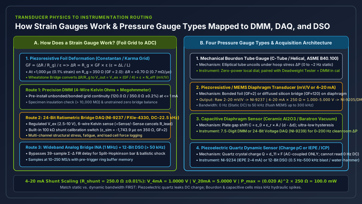
| Pressure Gauge Type | Physical Sensing Mechanism | Electrical Output Signal | Usable Frequency Bandwidth | Primary Target Instrument Architecture |
|---|---|---|---|---|
1. Mechanical Bourdon Tube Gauge (C-Tube, Helical, Spiral, ASME B40.100) |
Flattened elliptical metal tube (316L SS, phosphor bronze, Monel) uncoils under internal hoop stress ΔP, driving a sector-and-pinion pointer across a 270° dial (±0.1% Grade 4A to ±0.5% Grade 2A). |
None (0 W local visual dial, unless fitted with limit contacts or LVDT transmitter). |
0 Hz (Static) to ~2 Hz (rapid pulsation causes gear wear and requires glycerine fill + snubber). |
Zero-power local safety indicator; paired with a pneumatic/hydraulic deadweight tester and Precision DMM when calibrating electronic transmitters. |
| 2. Piezoresistive / Strain-Gauge Diaphragm Transducer (Bonded Foil or MEMS Silicon) | Pressure deflects an elastic steel or monocrystalline silicon diaphragm containing a 4-active-arm Wheatstone bridge (GF ≈ 2 sputtered metal foil or GF ≈ 100–150 diffused p-type silicon). |
Unconditioned: 2 to 20 mV/V ratiometric bridge. Conditioned industrial transmitter: 4–20 mA current loop, 0–5 V, or 0–10 V DC. |
0 Hz (Static DC) to 1 kHz – 50 kHz (flush miniature MEMS sensors reach 100–300 kHz). |
Raw mV/V bridges -> 24-Bit Bridge DAQ (NI-9237). Conditioned 4–20 mA loops -> Current DAQ (NI-9203), 16-Bit SAR DAQ (NI-9205 + external precision shunt), or DMM. |
3. Capacitive Diaphragm Pressure Sensor (Ceramic Al2O3 or Metal Baratron Cell) |
Pressure bows a taut ceramic or Inconel diaphragm toward a fixed electrode (C = ε_0 × ε_r × A / (d - Δd)), shifting capacitance by picofarads on a 50–100 pF baseline digitized by an internal AC ASIC. |
Conditioned 0–10 V DC, 0–5 V DC, 4–20 mA (with HART FSK), or digital RS-485. |
0 Hz (Static DC) to 20 Hz – 200 Hz (optimized for ultra-low hysteresis and vacuum/draft stability). |
6.5–7.5 Digit DMM (NI PXIe-4081) or 24-Bit Voltage DAQ (NI-9239) for semiconductor vacuum, cleanroom draft ΔP, and 0.025% custody-transfer flow calibration. |
4. Piezoelectric Dynamic Pressure Sensor (Quartz SiO2 or Tourmaline Crystal) |
Dynamic pressure ΔP(t) stresses a rigid crystal lattice, generating electrostatic charge Q = d_11 × F (pC/psi). Charge leaks through finite insulation resistance (τ = R_f × C_f), so it cannot read steady DC pressure. |
Charge mode (pC into external charge amp) or IEPE / ICP mode (2–20 mA @ 18–30 VDC constant-current excitation over BNC coax, ±5 V AC-coupled on ~10 VDC bias). |
0.5 Hz (AC-coupled high-pass) up to 100 kHz – 500 kHz (< 1 μs rise time). |
24-Bit IEPE Dynamic Signal DAQ (NI-9234 with built-in 2–4 mA IEPE source and AC coupling) up to 51.2 kS/s, or 12-Bit DSO (10 MS/s–1 GS/s) for hydraulic water-hammer, combustion knock, and blast shockwaves. |
Worked Example 4: Scaling a 4–20 mA Piezoresistive Pressure Transmitter Across a Precision Shunt
As detailed in our 4–20 mA sensor DAQ wiring and shunt check guide and the National Instruments Current Measurements Guide, connecting an industrial 0 to 100 bar (0 to 1,450 psi) two-wire 4–20 mA piezoresistive pressure transmitter to a voltage-input DMM or 16-bit SAR DAQ (NI-9205) requires converting loop current I_loop into voltage via a precision four-terminal or low-TCR shunt resistor R_shunt (±0.01% tolerance, <= 5 to 15 ppm/°C):
Given:
• Pressure range: P_min = 0.00 bar (at I_min = 4.000 mA), P_max = 100.00 bar (at I_max = 20.000 mA)
• Useful current span: ΔI = 20.000 mA - 4.000 mA = 16.000 mA
• External precision shunt resistor: R_shunt = 250.00 Ω (±0.01%, 0.5 W metal foil)
  (Note: A 249.00 Ω ±0.1% EIA standard resistor yields 0.996 V to 4.980 V to stay safely inside a ±5.00 V ADC clip limit.)

1. Ohm's Law Voltage Conversion (V_shunt = I_loop × R_shunt):
   • At 0.00 bar (4.000 mA live zero):  V_min  = 0.004000 A × 250.00 Ω = 1.0000 V
   • At 100.00 bar (20.000 mA FS):      V_max  = 0.020000 A × 250.00 Ω = 5.0000 V
   • At broken cable / fault (0.00 mA): V_fault = 0.0000 V (immediately distinguishable from 0.00 bar live zero!)
   • Linear pressure scaling equation:  P(bar) = 100.00 × (V_measured - 1.0000 V) / (5.0000 V - 1.0000 V)
                                               = 25.00 bar/V × (V_measured - 1.0000 V)

2. Shunt Resistor Self-Heating Power Check:
   • Maximum continuous power at 20.000 mA: P_shunt = I_max^2 × R_shunt = (0.020 A)^2 × 250.0 Ω = 0.100 W (100.0 mW)
   • Use at least a 0.50 W or 1.0 W rated precision foil resistor so self-heating temperature rise stays < 2°C.

3. Resolution Comparison Across Target Instruments (over the 4.0000 V active span):
   • 6.5-Digit DMM (10 V range, 1 NPLC): Resolves 10 μV steps => 0.00025 bar (0.25 mbar) with ±0.015% loop accuracy.
   • 16-Bit SAR DAQ (NI-9205 on ±5 V range, V_FSR = 10 V, V_LSB = 152.6 μV): Resolves 0.0038 bar (3.8 mbar) per LSB.
   • 8-Bit Oscilloscope (on 1 V/div × 8 div = 8 V span, 6.2 ENOB => V_res_eff = 108.8 mV):
     Resolves only 2.72 bar steps (2.7% of full scale), making an 8-bit scope unsuitable for static loop calibration.
When scanning multiple 4–20 mA shunt channels alongside high-impedance voltage sensors on a multiplexed SAR DAQ (NI-9205), ensure the source impedance seen by the analog multiplexer stays below 1 kΩ (which R_shunt = 250 Ω satisfies easily) to prevent inter-channel charge-injection crosstalk as detailed in our multiplexed DAQ ghosting test checklist.
Takeaway: Match the pressure transducer’s physical mechanism to the instrument input: route static and low-frequency piezoresistive (mV/V or 4–20 mA) and capacitive gauges to ratiometric or shunt-equipped DAQs and DMMs, and reserve IEPE dynamic inputs (NI-9234) or triggered oscilloscopes for AC-coupled piezoelectric quartz sensors.
How Should You Architect a Hybrid PXIe or Benchtop Automated Test System?
In production functional test and R&D validation racks (categorized under test and measurement), trying to force one instrument class to execute every measurement either degrades test accuracy or inflates hardware cost. A well-architected PXIe or hybrid LXI/CompactDAQ test bench assigns each signal to its native converter domain and links them via hardware trigger buses (PXI_Trig0..7 or PFI lines). For multi-channel sample rate and disk throughput budgeting across long test runs, use our DAQ sample rate planning worksheet.
5-Step Test Bench Channel Assignment Checklist
- Separate continuous logs from triggered windows first: Write two separate specification lines if a channel requires both a continuous multi-hour trend file and a nanosecond pre-trigger fault capture, following the acceptance tests in our DAQ vs oscilloscope guide.
- Audit every probe and terminal for common-mode voltage (
V_CM) and earth ground: Identify every measurement point that does not sit at0.0 VProtective Earth (high-side shunts,Wheatstone bridge midpoints,floating battery cells). Ban passive earth-grounded oscilloscope BNC probes on those nodes; assign them to aCAT IIfloating DMM, an isolated differential DAQ (NI-9237,NI-9239), or an active HV differential scope probe. - Check required vertical resolution (
V_res_eff) against IEEE Std 1241ENOB: ComputeV_res_eff = V_FSR / 2^ENOBon the chosen input range. Route any channel requiring< 100 μVabsolute accuracy, four-wire Kelvin resistance, or>= 60 dB50/60 Hzmains rejection to a6.5–7.5 digitDMM running at>= 1 NPLC(100 msuniversal window for global deployment). - Group synchronized sensor arrays onto dedicated conditioned DAQ modules: Land full/half/quarter strain bridges on
24-bitratiometric modules (NI-9237) with 6-wire Kelvin remote sense and100 kΩshunt verification; land4–20 mAindustrial pressure transmitters on current/shunt DAQ channels (NI-9203orNI-9205with250 Ω ±0.01%shunts); land dynamic piezoelectric sensors on AC-coupled IEPE DSA modules (NI-9234). - Cross-trigger the oscilloscope from the DAQ or DMM limit comparator: When investigating intermittent electromechanical faults, configure the multi-channel DAQ or DMM hardware comparator to assert a digital TTL trigger pulse over the backplane (
PXI_Trig/PFI0) the instant strain, pressure, or supply current crosses a fault threshold, freezing the oscilloscope’s circular pre-trigger ring buffer around the exact microsecond of failure.
Takeaway: Build your automated test bench by combining the 24-bit ratiometric conditioning of modular DAQ, the 100 ms line-locked ppm accuracy of a floating DMM, and the gigasample pre-trigger memory of a digital oscilloscope linked over a shared hardware trigger line.