Strain Gage Accuracy Error Budget: Gage Factor, Thermal Output, and Leadwire Corrections

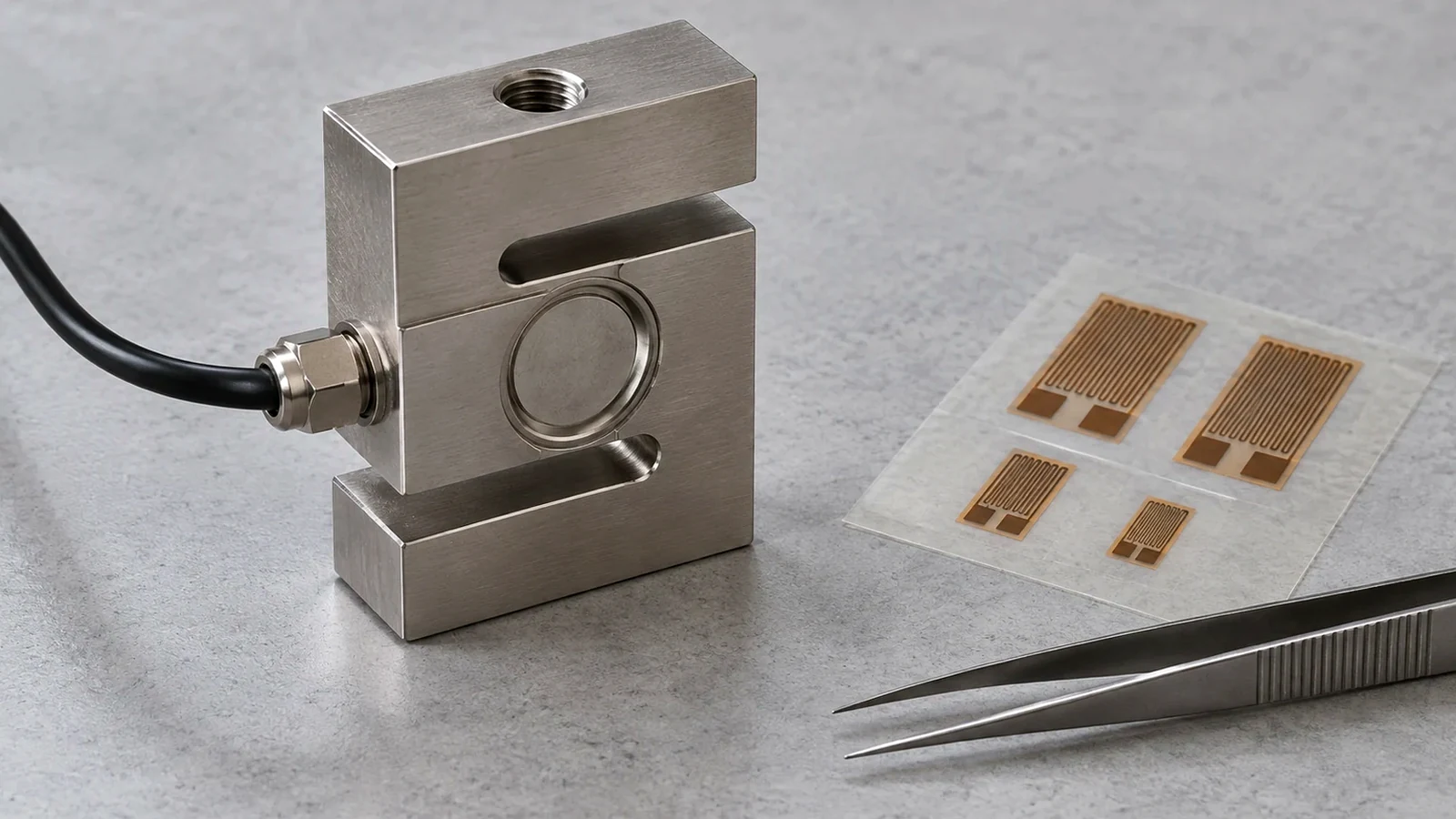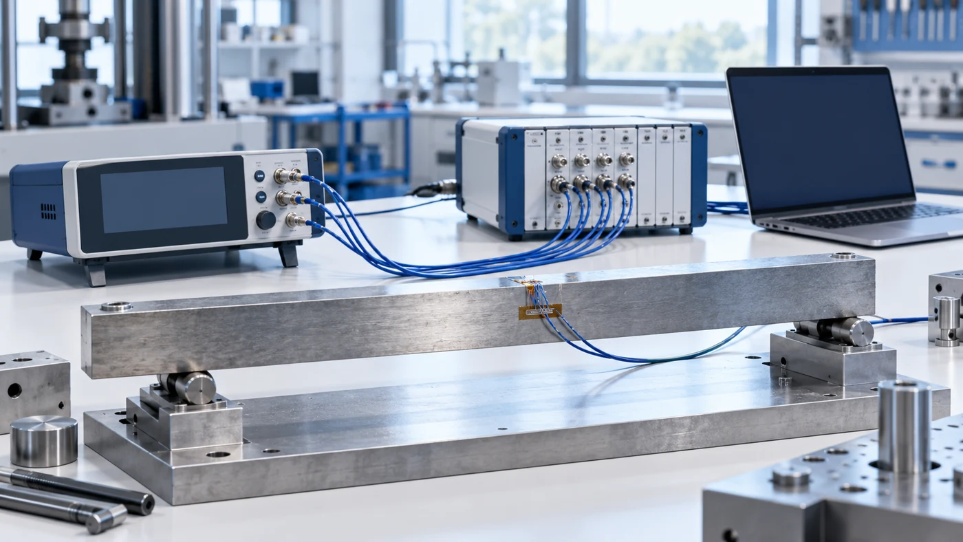
Relying on software offset compensation alone leaves the physical offset of a Wheatstone bridge intact, which if large enough limits amplifier gain and dynamic range. Under ASTM E251-20a Clauses 1.3.2 and 1.3.5, the accuracy of strain gage data can be no better than the accuracy of the gage factor, while thermal output acts as an additive (not multiplicative) error that can often be much larger than the strain gage output from structural loading.

Engineers evaluating how to measure strain using strain gauge instrumentation across our sensors and DAQ engineering guides must account for every error mechanism between the bonded foil grid and the analog-to-digital converter. ASTM E251-20a (Clause 1.2) defines standard test methods for determining five metallic bonded resistance strain gage performance characteristics: Resistance at a Reference Temperature (Section 8), Gage Factor at a Reference Temperature (Section 9), Temperature Coefficient of Gage Factor (Section 10), Transverse Sensitivity (Section 11), and Thermal Output (Section 12). Under Clauses 1.4 and 1.5, metallic bonded resistance strain gages measure average unit elongation (ΔL/L) over a nominal gauge length so Practice E83 is not applicable to them, and these test methods do not apply to transducers such as load cells and extensometers.

In Vishay Micro-Measurements Tech Note TN-505-4 selection tables, general stress-analysis strain gauge accuracy categories are defined as 2 to 5% for moderate accuracy, 1 to 3% for high accuracy, and 1% or better for very high accuracy, whereas transducer gaging achieves better than 0.2% with N2A series gages (-50° to +200°F [-45° to +95°C]), 0.2 to 0.5% with WA and SA series gages (-50° to +300°F [-45° to +150°C]), and better than 0.5% with WK and SK series gages (-320° to +350°F [-195° to +175°C]). Reaching the 1 to 3% high-accuracy stress-analysis category requires deconstructing the error budget into gage factor tolerance and temperature drift, thermal output (apparent strain), leadwire resistance desensitization, and secondary bridge and instrumentation effects.

Error Budget Term	Error Classification	Governing Equation or Mechanism	Representative Uncorrected Magnitude
Gage factor lot tolerance	Multiplicative scale error	Transfer function accuracy limit under ASTM E251-20a Clause 1.3.2; statistical lot testing under Clauses 4.2 and 4.3	±1% gage factor tolerance on a 350-ohm gage (gage factor 2.0) shunted for 2000 με contributes to ±2.23% combined root-sum-square uncertainty
Gage factor temperature variation	Multiplicative scale drift	F2 = F1 × (1 + ΔF / 100) and ε2 = ε1 × (F1 / F2)	typically in the order of 1% or less per 100°F [2% or less per 100°C] for constantan (A-alloy), with package data showing (+1.1 ±0.2)%/100°C
Thermal output (apparent strain)	Additive zero shift	ε_T/O = A0 + A1 T + A2 T^2 + A3 T^3 + A4 T^4 adjusted by 2.0 / FI	Residual error on the order of 10 me/°C with self-temperature-compensated gage alone; reduced to as small as 1 me/°C with fourth-order polynomial correction
Two-wire leadwire resistance and thermal drift	Additive drift and multiplicative attenuation	Series lead resistance in active quarter-bridge arm; copper resistance changes by approximately 22% per 100°F [55°C]	20-ft [6 m] of AWG26 [0.4 mm dia.] copper wire (1.7 ohms) on a 120-ohm gage (gage factor 2.0) causes 7000 με imbalance, 1.5% sensitivity loss, and 156 microstrain (4700 psi [0.03 GPa] in steel) per 10°F [5.5°C]
Three-wire leadwire desensitization	Multiplicative scale attenuation	Equal leadwires RL1 and RL2 in adjacent arms; signal attenuated by RG / (RG + RL)	Desensitization reduced by about 50% compared to two-wire circuit; Quarter-Bridge Type I software conversion multiplies by (1 + RL / Rg)
Unbalanced quarter-bridge nonlinearity	Nonlinear scale error	Unbalanced quarter-bridge Wheatstone circuit (TN-507-1 Section 1.0)	Percentage nonlinearity error is approximately equal to strain in percent: about 0.1% at 1000 με, 1% at 10,000 με, and 10% at 100,000 με

Why Balancing a Wheatstone Bridge Does Not Equal Calibration

A foundational principle of strain gauge basics is that metallic foil grids convert minute mechanical deformations into micro-ohm to milli-ohm resistance shifts. For a typical commercial strain gage with resistance R = 120 Ω (or 350 Ω) and strain gage factor S around 2.0 over a typical metal-beam axial strain range of 10^-6 to 10^-3, the resistance change δR is between 0.00024 Ω and 0.24 Ω, which corresponds to a fractional resistance change δR/R of 2 × 10^-6 to 2 × 10^-3. In a balanced quarter-bridge circuit with strain gage factor S = 2.0 and excitation supply voltage Vs = 5.00 V, a measured output voltage Vo = 1.13 mV (with 1000 mV per 1 V) corresponds to an axial strain of 0.000452, or 452 μstrain (450 μstrain to two significant digits).

Slight variations in bridge-arm and lead resistance, plus a prestrained installation, create an initial non-zero bridge output before mechanical load is applied, so data acquisition systems provide bridge balancing (offset nulling) routines. Software offset compensation takes an initial measurement before applying strain input and uses this offset in the strain conversion equations, but does not remove the physical offset of the bridge, which if large enough limits the amplifier gain and dynamic range of the measurement. Hardware bridge balancing uses either an offset-nulling potentiometer circuit to physically adjust bridge output to zero volts, or buffered offset nulling that adds an adjustable positive or negative DC voltage to the instrumentation amplifier output. On the NI SCXI-1520 strain module, offset null compensation provides a range of ±4% of excitation voltage with 20,000 counts of resolution, corresponding to a ±80,000 με offset null compensation range and 4 με resolution for a quarter-bridge with GF = 2.0.

Zeroing the bridge only establishes a baseline reference at the instant of nulling; it neither verifies the electrical gain of the signal chain nor compensates for temperature shifts after nulling. Unlike offset nulling, shunt calibration connects a known resistor across one bridge leg to obtain a gain adjust factor (defined as simulated signal level divided by measured signal level with the shunt resistor engaged) that corrects for system gain error and discrepancies between nominal Gauge Factor and actual Gauge Factor. Even after shunt calibration, the conversion from bridge voltage to actual mechanical strain remains governed by the three primary correction terms in strain gage theory: gage factor tolerance and temperature variation, thermal output, and leadwire resistance effects.

First Error Term: Gage Factor Lot Tolerance and Temperature Variation

Under ASTM E251-20a Clause 1.3.2, gage factor is the transfer function of a strain gage relating resistance change in the strain gage and the strain to which it is subjected, and the accuracy of strain gage data can be no better than the accuracy of the gage factor. Under Clauses 4.2 and 4.3, most performance characteristics of strain gages require destructive mechanical testing so data must be treated statistically by lot or batch, and individual strain gages cannot be calibrated, whereas resistance measurement is non-destructive and can be made for each strain gage.

That statistical lot uncertainty propagates directly into shunt calibration and strain scaling. In Vishay Micro-Measurements Tech Note TN-514 uncertainty propagation (Equation 45), shunting a 350-ohm gage (having a gage factor of 2.0, ±1% gage factor tolerance, ±0.3% package resistance tolerance, and ±1% installed resistance uncertainty) with a shunt resistor RC = 87,150 ohms (±0.01% tolerance) to simulate 2000 με yields a combined root-sum-square uncertainty U_εS/εS = ±2.23%.

When test temperatures depart from room temperature, the gage factor itself shifts. For constantan (A-alloy) strain gages, the gage factor variation with temperature is essentially linear and typically in the order of 1% or less per 100°F [2% or less per 100°C], with package data showing Temperature Coefficient of Gage Factor = (+1.1 ±0.2)%/100°C. To correct strain data for gage factor variation with temperature, the test-temperature gage factor is F2 = F1 × (1 + ΔF/100) and the corrected strain is ε2 = ε1 × (F1 / F2); for a 13 S-T-C K-alloy gage with room-temperature gage factor F1 = 2.05 at +450°F [+230°C] where ΔF is -3 (or -0.03), F2 = 2.05 × (1 - 0.03) = 1.99 and an indicated strain of 1820 με corrects to 1875 με.

Second Error Term: Thermal Output (Apparent Strain) and S-T-C Matching

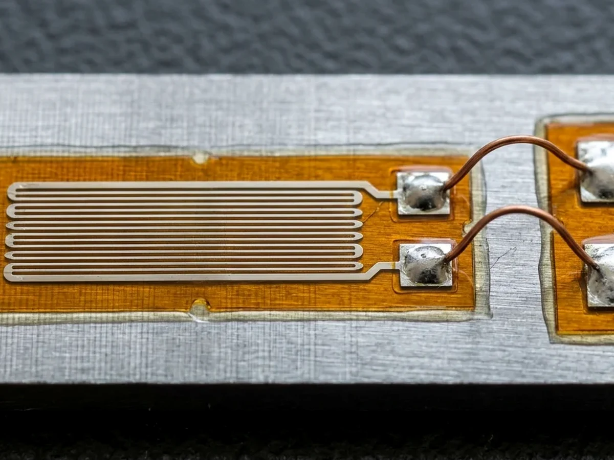
Under ASTM E251-20a Clause 1.3.5, thermal output is the response of a strain gage to temperature changes and is an additive (not multiplicative) error that can often be much larger than the strain gage output from structural loading. In Tech Note TN-504-1, Eq.(1) gives (ΔR/R)T/O from the grid temperature coefficient of resistance, the gage factor FG, the transverse sensitivity factor (1 + Kt)/(1 - ν0 Kt) where Poisson’s ratio ν0 is 0.285, and the differential thermal expansion (αS - αG) ΔT between specimen and grid; Eq.(2) divides that by the instrument gage factor setting FI to express thermal output in strain units.

Self-temperature-compensated constantan (A-alloy) and modified Karma (K-alloy) strain gages are specially processed to produce minimum thermal output over the temperature range from about -50° to +400°F [-45° to +200°C], whereas uncompensated isoelastic (D alloy, gage factor approximately 3.2) exhibits a thermal output of about 80 με/°F [145 με/°C]. Micro-Measurements constantan alloy gages are available in S-T-C numbers 00, 03, 05, 06, 09, 13, 15, 18, 30, 40, and 50 (with 30 and higher intended primarily for plastics), while K-alloy gages are available in S-T-C numbers 00, 03, 05, 06, 09, 13, and 15. In Table 1 of TN-504-1, nominal thermal expansion coefficients (per °F [per °C]) and recommended S-T-C numbers for standard reference test materials include 6.7 [12.1] with S-T-C 06 for 1008, 1018 carbon steel and 9.6 [17.3] with S-T-C 09 for 304 austenitic stainless steel. In the same reference table, nominal thermal expansion coefficients (per °F [per °C]) and recommended S-T-C numbers are 6.4 [11.5] with S-T-C 06 for pure beryllium, 11.1 [20.0] with S-T-C 13 for cartridge brass, and 14.5 [26.1] with S-T-C 15 for AZ-31B magnesium alloy.

Matching the S-T-C number to the test specimen does not make thermal output zero across a wide temperature excursion. When using a self-temperature-compensated strain gage without software curve correction, a residual thermal error on the order of 10 me/°C is still possible, whereas conducting software temperature correction with the fourth-order polynomial coefficients printed on the gage package can reduce the error to as small as 1 me/°C. For computerized thermal output correction, Micro-Measurements supplies for each lot of A-alloy and K-alloy gages a fourth-order least-squares polynomial ε_T/O = A0 + A1 T + A2 T^2 + A3 T^3 + A4 T^4 (Equation 5); in the Figure 5 package example tested on 2024-T4 aluminum, the Fahrenheit polynomial is ε_TO = -8.82×10^1 + 2.71×10^0 T - 2.53×10^-2 T^2 + 6.72×10^-5 T^3 - 4.03×10^-8 T^4.

Because Micro-Measurements thermal output data are standardized at an instrument gage factor FI = 2.0 for A- and K-alloy gages, setting the instrument to FI ≠ 2.0 requires scaling the published thermal output by ε’_T/O = ε_T/O × (2.0 / FI) (Equation 4); at +250°F [+121°C] where ε_T/O is -100 με and FI = 2.10, the adjusted thermal output ε’_T/O is -95 με, so an indicated strain of +2300 με corrects to 2300 - (-95) = 2395 με (and -2300 με corrects to -2205 με). When both thermal output and gage factor temperature variation must be corrected simultaneously after balancing the instrument at room temperature with FI = F* = 2.0 (Equation 11), the corrected strain is ε1 = [ε_hat1 - ε_T/O(T1)] × (F* / F(T1)); for a WK-06-250BG-350 gage on steel at T1 = -50°F [-45°C] with room-temperature gage factor F0 = 2.07, ΔF(T1) = +0.6% (giving F(T1) = 2.08), ε_T/O(T1) = -200 με, and an uncorrected reading of -1850 με, the corrected strain is [-1850 - (-200)] × (2.0 / 2.08) = -1587 με.

Third Error Term: Leadwire Resistance Desensitization and Thermal Drift

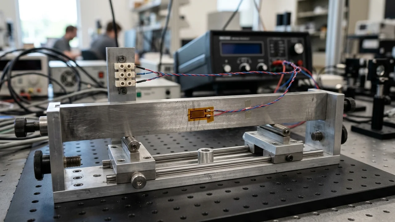
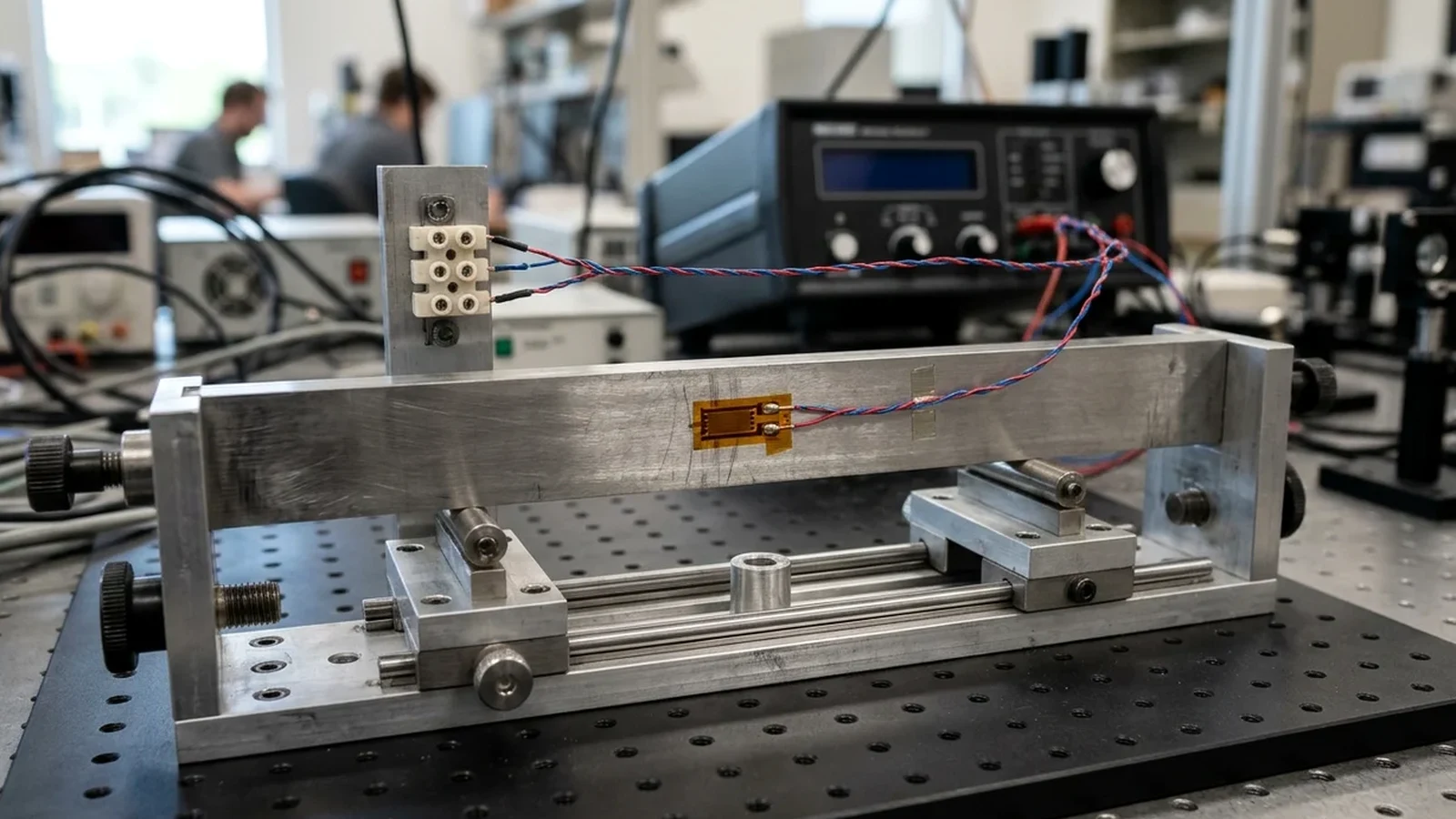
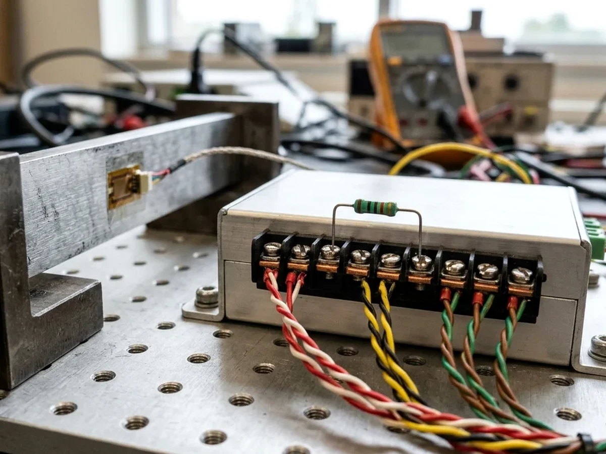
In a two-wire quarter-bridge Wheatstone configuration, parasitic leadwire resistance between the instrumentation terminal block and the strain gage introduces both zero drift and span attenuation. In a two-wire quarter-bridge circuit with a 120-ohm strain gage (gage factor setting 2.0), a 20-ft [6 m] length of two-conductor AWG26 [0.4 mm dia.] copper leadwire has a room-temperature resistance of about 1.7 ohms and produces an initial bridge imbalance of about 7000 με, about a 1.5% loss in sensitivity, and a leadwire thermal drift error of approximately 156 microstrain (about 4700 psi [0.03 GPa] in steel) per 10°F [5.5°C] temperature change, because copper resistance changes by approximately 22% per 100°F [55°C].

In a three-wire quarter-bridge circuit, equal leadwires RL1 and RL2 are placed in adjacent bridge arms so the bridge remains in balance during leadwire temperature changes, and because only one leadwire is in series with the strain gage, leadwire desensitization is reduced by about 50% compared to the two-wire configuration. However, in a three-wire quarter-bridge circuit, the strain signal is still attenuated (desensitized) by the factor RG / (RG + RL), where RL is the resistance of one leadwire in series with the active gage resistance RG (TN-514 Section III). Readers performing field installation verification can follow our guide on three-wire quarter-bridge resistance checks before energizing the bridge.

For Quarter-Bridge Type I on the NI SCXI-1520, the voltage drop across lead resistance RL is uncompensated in hardware and the software conversion equation multiplies by (1 + RL/Rg), where 10 ft of 24-AWG copper wire has a lead resistance RL of 0.25 Ω and quarter-bridge completion uses a 0.1% precision dummy resistor; the active gage should use STC = 13.0 on aluminum or STC = 6.0 on steel. In a full-bridge configuration without remote sense and without shunt calibration, measurements must be multiplied by the Gain Adjusting Factor = 1 + (2 × RL / Rg) to compensate for the excitation voltage drop across the lead resistance.

Gage resistance and factory cable selection also shape the leadwire error budget. Selecting a 350-ohm strain gage over a 120-ohm strain gage reduces the heat generation rate by a factor of three for the same applied voltage across the gage and decreases leadwire desensitization and thermal lead effects. When gages are ordered with factory-attached leads, Micro-Measurements Option P preattached 10-ft [3.1 m] three-conductor 26-gauge [0.404 mm dia.] vinyl-insulated copper cable has a nominal resistance of 0.04 ohm/ft [0.13 ohm/m] per conductor, whereas Option P2 preattached cable on CEA-Series gages has a nominal resistance of 0.11 ohm/ft [0.36 ohm/m] per conductor, and in both options gage resistance is measured at the gage tabs and gage factor is determined without preattached cable. To empirically calibrate out leadwire attenuation via shunt calibration across the active arm, TN-514 Table 1 (based on circuit gage factor 2.000 and ±0.02% precision shunt resistors) specifies that for a 120-ohm gage a 59,880-ohm shunt resistor simulates 1000 microstrain and 29,880 ohms simulates 2000 microstrain, while for a 350-ohm gage an 87,150-ohm resistor simulates 2000 microstrain.

Secondary Error Contributors: Nonlinearity, Excitation Heating, Transverse Sensitivity, and DAQ Stability

Beyond the three primary correction equations, high-precision structural and materials testing must budget for four additional error sources:

1. Wheatstone Bridge Nonlinearity: In an unbalanced quarter-bridge Wheatstone circuit, percentage nonlinearity error is approximately equal to the strain in percent: about 0.1% at 1000 με, 1% at 10,000 με, and 10% at 100,000 με (TN-507-1 Section 1.0). In a half-bridge circuit where two series arms undergo equal and opposite resistance changes (ε2 = -ε1, such as a beam in bending), the nonlinearity terms in the denominator cancel and the bridge output is strictly linear: Δ(eO/E) = FG × ε / 2; however, shunting a single arm during shunt calibration always results in nonlinear quarter-bridge operation Δ(eO/E) = FG × ε / (4 + 2 × FG × ε).
2. Excitation Self-Heating and Rosette Derating: A full-bridge four-active-element strain gauge configuration doubles bending measurement sensitivity compared with a half-bridge implementation, whereas increasing excitation voltage increases power dissipation by the square of voltage and makes the gauge susceptible to self-heating thermal error. For an equal-arm Wheatstone bridge with bridge excitation voltage EB, active gage resistance RG, and grid area AG, grid power density P’G = PG / AG relates to bridge voltage by EB = 2 × sqrt(RG × P’G × AG), and under high-accuracy static requirements TN-502 Table 1 specifies power density levels (in watts/in^2 [kilowatts/m^2]) of 2–5 [3.1–7.8] on heavy aluminum or copper, 1–2 [1.6–3.1] on thick steel, 0.5–1 [0.78–1.6] on thin stainless steel or titanium, 0.1–0.2 [0.16–0.31] on filled plastic, and 0.01–0.02 on unfilled plastic. For a three-element stacked rosette where all three grids are completely superimposed and receive equal input power, the top grid experiences six times the temperature rise of a similar single gage, so each rosette grid should receive 1/6 of the single-gage power (a bridge excitation voltage reduction factor of 2.5); for a two-element stacked rosette, the power derating factor is 3 and the bridge voltage reduction factor is 1.7.
3. Transverse Sensitivity and Gage Length Selection: Under ASTM E251-20a Clause 1.3.4, transverse sensitivity is a measure of the strain gage response to strains perpendicular to its measurement axis, and although it is usually much less than 10 % of the gage factor, large errors can occur if the value is not known with reasonable precision. As detailed in our companion article on strain gauge factor and transverse sensitivity, for any biaxial strain field with strains εa and εt parallel and perpendicular to the primary sensing axis, the percentage error n_ε due to transverse sensitivity Kt is n_ε = [Kt × ((εt/εa) + ν0) / (1 - ν0 × Kt)] × 100, where Kt = Ft / Fa (Equation 2). To avoid strain-averaging accuracy loss near a stress concentration (hole, fillet, or notch), TN-505-4 Section 2.4 specifies that the strain gage length should be no greater than 0.1 times the radius of a hole, fillet, or notch, or the corresponding dimension of any other stress raiser, whereas gages shorter than about 0.125 in [3 mm] tend to exhibit degraded static stability, maximum elongation, and cyclic endurance, making 0.125 to 0.25 in [3 to 6 mm] gage lengths generally preferable.
4. DAQ Signal Conditioning Stability and Noise Rejection: On the NI SCXI-1520 strain module (Appendix A Specifications), recommended warm-up time is 15 minutes, maximum gain drift is ±40 ppm of reading/°C, and offset drift is ±2 μV/°C typical (±5 μV/°C max) for Gain ≥20 and ±10 μV/°C typical (±25 μV/°C max) for Gain <20. Constant-voltage excitation on the NI SCXI-1520 is configurable from 0.0 to 10.0 V in 0.625 V increments with a maximum operating current of 29 mA in all ranges, load regulation (no load to 120 Ω load) of ±0.003% with remote sense versus ±0.08% without remote sense, excitation temperature drift of ±0.005%/°C (±30 μV/°C max), remote sense error less than ±0.02% per ohm of lead resistance (both leads), and internal half-bridge completion using two 5 kΩ precision resistors with 0.1% ratio matching. Finally, a data acquisition measurement device with a spurious-free dynamic range (SFDR) of 106 dB is equivalent to noise levels of about 0.0005 percent of the full input range, while power line interference commonly appears as 50 Hz or 60 Hz noise.

For more information on how we review and document measurement engineering workflows, visit our editorial methodology and about page. Maximizing Value at NI is an independent technical resource and is not affiliated with National Instruments or Emerson.

Sources

• ASTM International — Standard Test Methods for Performance Characteristics of Metallic Bonded Resistance Strain Gages
• Vishay Micro-Measurements — Strain Gage Thermal Output and Gage Factor Variation with Temperature
• Vishay Micro-Measurements — Strain Gage Selection: Criteria, Procedures, Recommendations
• Vishay Micro-Measurements — Shunt Calibration of Strain Gage Instrumentation
• Vishay Micro-Measurements — The Three-Wire Quarter-Bridge Circuit
• Vishay Micro-Measurements — Optimizing Strain Gage Excitation Levels
• Vishay Micro-Measurements — Errors Due to Wheatstone Bridge Nonlinearity
• Vishay Micro-Measurements — Errors Due to Transverse Sensitivity in Strain Gages
• National Instruments — Engineer’s Guide to Accurate Sensor Measurements
• National Instruments — Strain Conditioning Module User Manual
• Penn State University Mechanical Engineering Lecture Notes — Stress, Strain, and Strain Gages